When I get into a dispute about how digital audio works, I’ll often be the guy making the bizarre and counter-intuitive statements:

“Bit depth affects the noise floor, not the ability to reproduce a wave-shape accurately.”

“Sample rates beyond 44.1 k don’t make material below 21 kHz more accurate.”

The thing is, I drop these bombshells without any experimental proof. It’s no wonder that I encounter a fair bit of pushback when I spout off about digital audio. The purpose of this article is to change that, because it simply isn’t fair for me to say something that runs counter to many people’s understanding…and then just walk away. Audio work, as artistic and subjective as it can be, is still governed by science – and good science demands experiments with reproducible results.

I Want You To Be Able To Participate

When I devised the tests that you’ll find in this article, one thing that I had in mind was that it should be easy for people to “try them at home.” For this reason, every experiment is conducted inside Reaper (a digital audio workstation), using audio processing that is available with the basic Reaper download.

Reaper isn’t free software, but you can download a completely un-crippled evaluation copy at reaper.fm. The 30-day trial period should be plenty of time for you to run these experiments yourself, and maybe even extend them.

To ensure that you can run everything, you will need to have audio hardware capable of a 96 kHz sampling rate. If you don’t, and you open one of the projects that specifies 96 kHz sampling, I’m not sure what will happen.

With the exception of Reaper itself, this ZIP file should contain everything you need to perform the experiments in this article.

IMPORTANT: You should NOT open any of these project files until you have turned the send level to your monitors or headphones down as far as possible. Otherwise, if I have forgotten to set the initial level of the master fader to “-inf,” you may get a VERY LOUD and unpleasant surprise. If you wreck your hearing or your gear in the process of experimenting, I am NOT responsible.

Weak Points In These Tests

The veracity of these experiments is by no means unassailable. It’s very important that I say that. For instance, the measurement “devices” that will be used are not independent of Reaper. They run inside the software itself, and so are subject to both their own flaws and the flaws of the host software.

Because I did not want to burden you with having to provide external hardware and software for testing, the only appeal to external measurement that is available is listening with the human ear. Human hearing, as an objective measurement, is highly fallible. Our ability to hear is not necessarily consistent across individuals, and what we hear can be altered by all manner of environmental factors that are directly or indirectly related to the digital signals being presented.

I personally hold these experiments as strong proof of my assertions, but I have no illusions of them being incontestable.

Getting Started – Why We Won’t Be Using Many “Null” Tests

A very common procedure for testing digital audio assumptions is the “null” test. This experiment involves taking two signals, inverting the polarity of one signal, and then summing the signals. If the signals are a perfect match, then the resulting summation will be digital silence. If they are not a perfect match, then some sort of differential signal will remain.

Null tests are great for proving some things, and not so great for proving others. The problem with appealing to a null test is that ANYTHING which changes anything about the signal will cause a differential “remainder” to appear. Because of this, you can’t use null testing to completely prove that, say, a 24-bit file and a 16-bit file contain the same desired signal, independent of noise. You CAN prove that the difference between the files is located at some level below 0 dBFS (decibels referenced to full scale), and you can make inferences as to the audibility of that difference. Still, the reality that the total signal (including unwanted noise) contained within a 16-bit file is different from the total signal contained within a 24-bit file is very real, and non-trivial.

There are other issues as well, which the first few experiments will reveal.

Open the project file that starts with “01,” verify that the master fader and your listening system are all the way down, and then begin playback. The analysis window should – within its own experimental error – show you a perfect, undistorted tone occurring at 10 kHz. As the file loops, there will be brief periods where noise becomes visible in the trace. Other than that, though, you should see something like this:

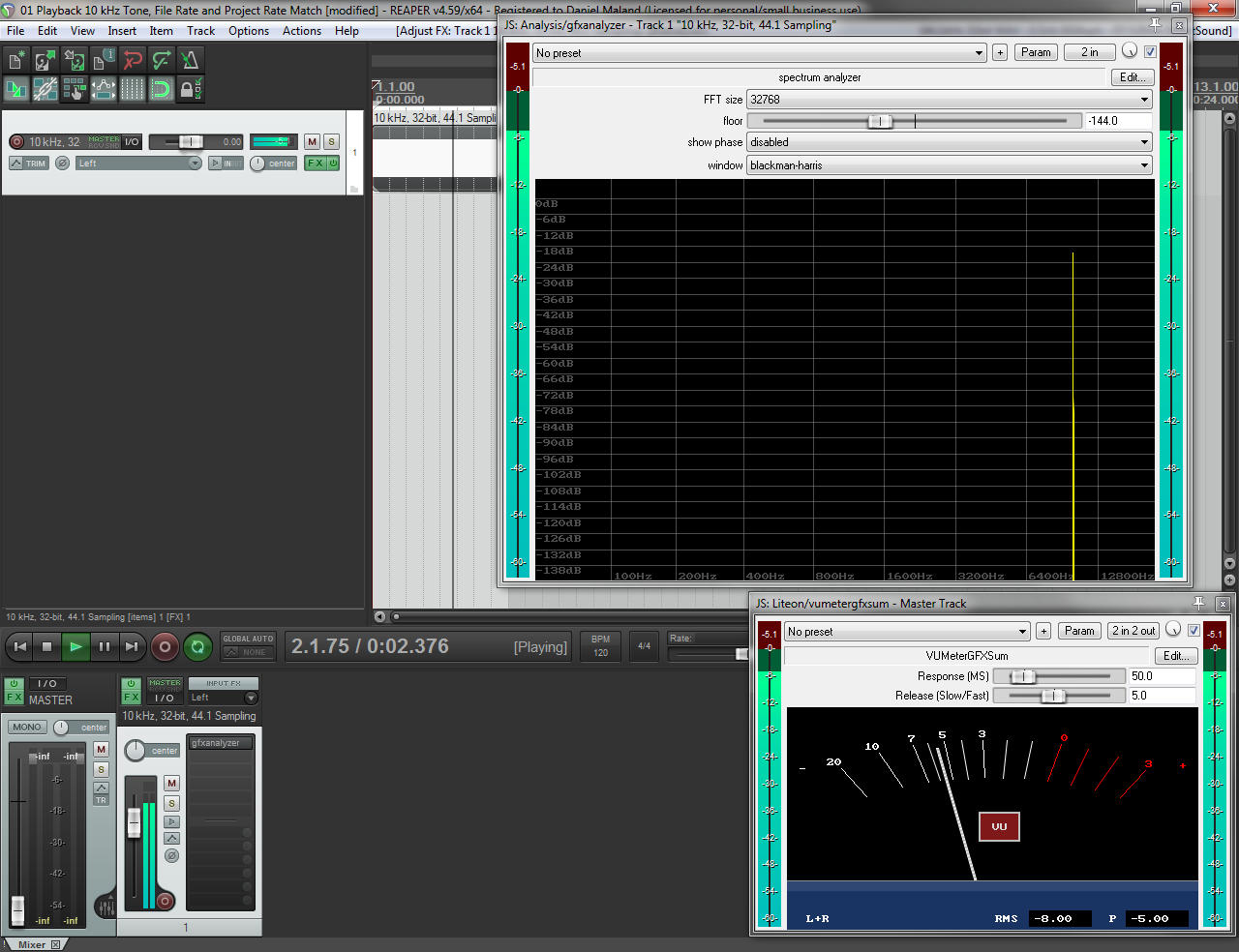
When Reaper is playing a file that is at the same sample rate as the project, nothing odd happens.

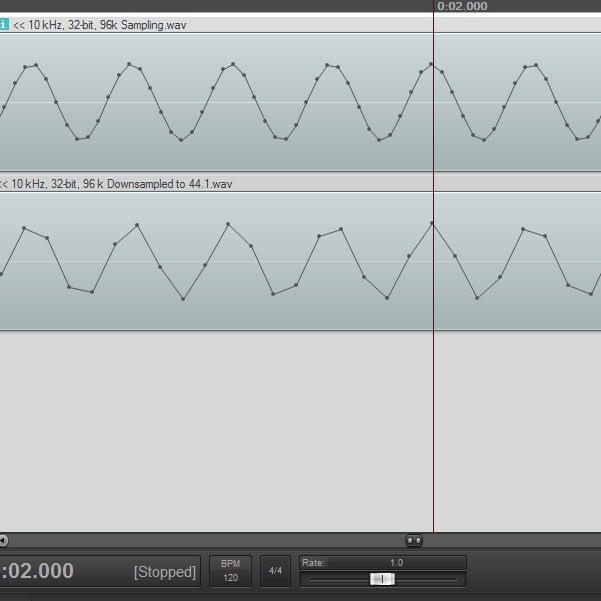
Now, open the file that starts with “02.” When you begin playback, something strange occurs. The file being played is the same one that was just being used, but this time the project should invoke a 96 kHz sample rate. As a result, Reaper will attempt to resample the file on the fly. This resampling results in some artifacts that are difficult (if not entirely impossible) to hear, but easy to see in the analyzer.

Reaper is incapable of realtime (or even non-realtime) resampling without artifacts, which means that we can’t use a null test to incontestably prove that a 10 kHz tone, sampled at 44.1 kHz, is exactly the same as a 10 kHz tone sampled at 96 kHz.

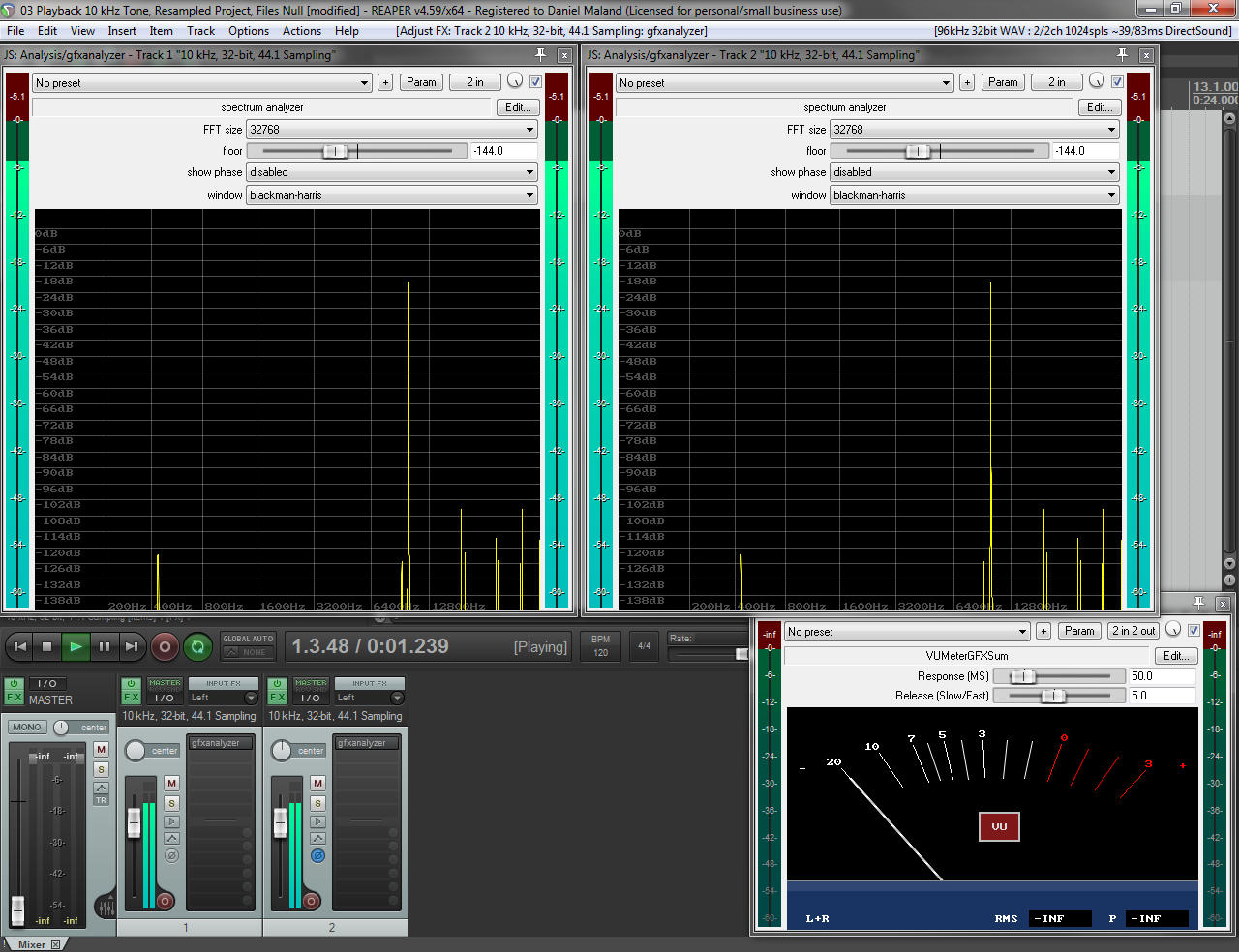
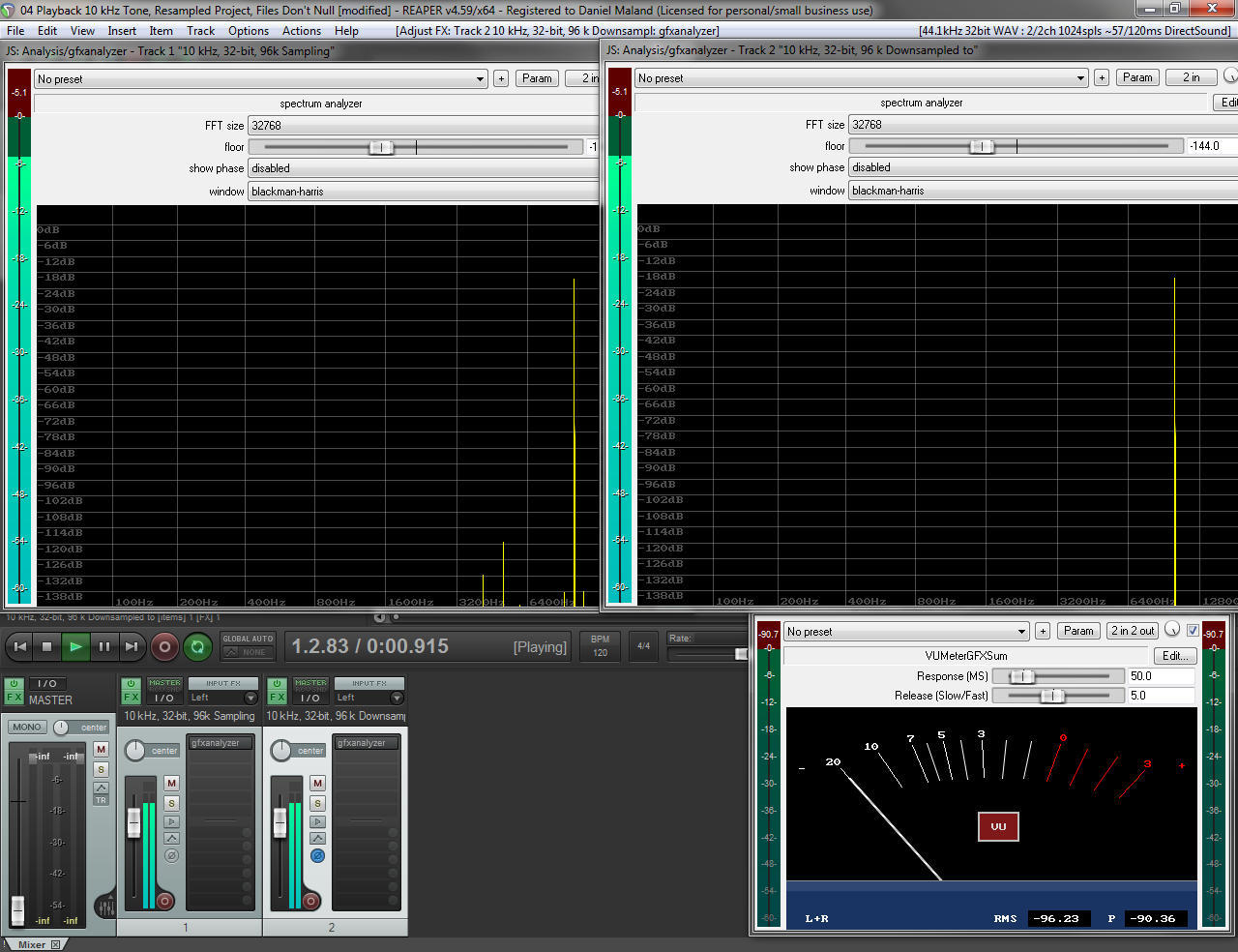
What is at least somewhat encouraging, though, is that the artifacts produced by Reaper’s resampling are consistent in time, and from channel to channel. Opening and playing the project starting with “03” confirms this, in a case where a null test is actually quite helpful. The same resampled file, played in two channels (with one channel polarity-inverted) creates a perfect null between itself and its counterpart.

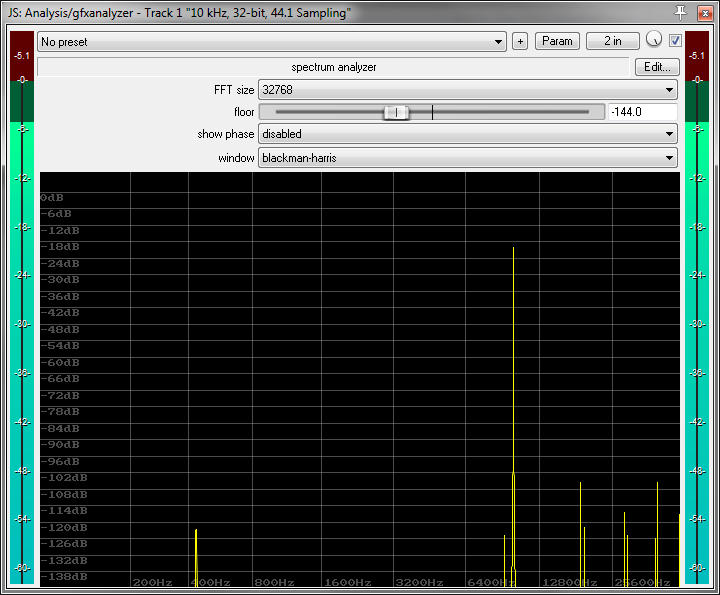
Test 04 demonstrates the problem that I talked about above. With one file played at the project’s “native” sample rate, and the other file being resampled, the inverted-polarity signal doesn’t null perfectly with the other channel. The differential signal IS a long way down, at about -90 dBFS. That’s probably impossible to hear under most normal circumstances, but it’s not digital silence.

Does A Higher Sampling Rate Render A Particular Tone More Accurately?

With the above experiments out of the way, we can now turn our attention to one of the major questions regarding digital audio: Does a higher rate of sampling, and thus, a more finely spaced “time grid,” result in a more accurate rendition of the source material?

Hypothesis 1: A higher rate of sampling does result in a more accurate rendition of a particular tone, as long as the tone in question is a frequency unaffected by input or output filtering. This hypothesis assumes that digital audio is an EXPLICIT representation of the signal – that is, that each sample point is reproduced “as is,” and so more samples per unit time create a more faithful reproduction of the material.

Hypothesis 2: A higher rate of sampling does not result in a more accurate rendition of a particular tone, as long as the tone in question is a frequency unaffected by input or output filtering. This hypothesis assumes that digital audio is an IMPLICIT representation of the signal, where the sample data is used to mathematically reconstruct a perfect copy of the stored event.

The experiment begins with the “05” project. The project generates a 10 kHz tone, with a 44.1 kHz sampling rate. If you listen to the output (and aren’t clipping anything) you should hear what the analyzer displays: A perfect, 10 kHz sine wave with no audible distortion, harmonics, undertones, or anything else.

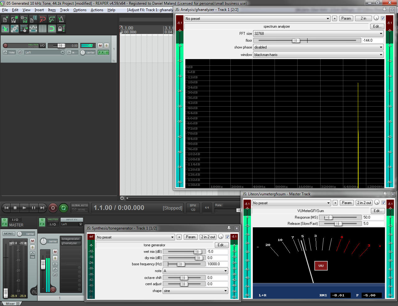
Project “06” generates the same tone, but in the context of a 96 kHz sampling rate. The analyzer shifts the trace to the left, because 96 kHz sampling can accommodate a wider frequency range. However, the signal content stays the same: We have a perfect, 10 kHz tone with no audible artifacts, and nothing else visible on the analyzer (within experimental error).

Project “07” also generates a 10 kHz tone, but it does so within a 22.05 kHz sampling rate. There is still no audible signal degradation, and the tone displays as “perfect” in the analyzer. The trace is shifted to the right, because 10 kHz is very near the limit of what 22.05 kHz sampling can handle.

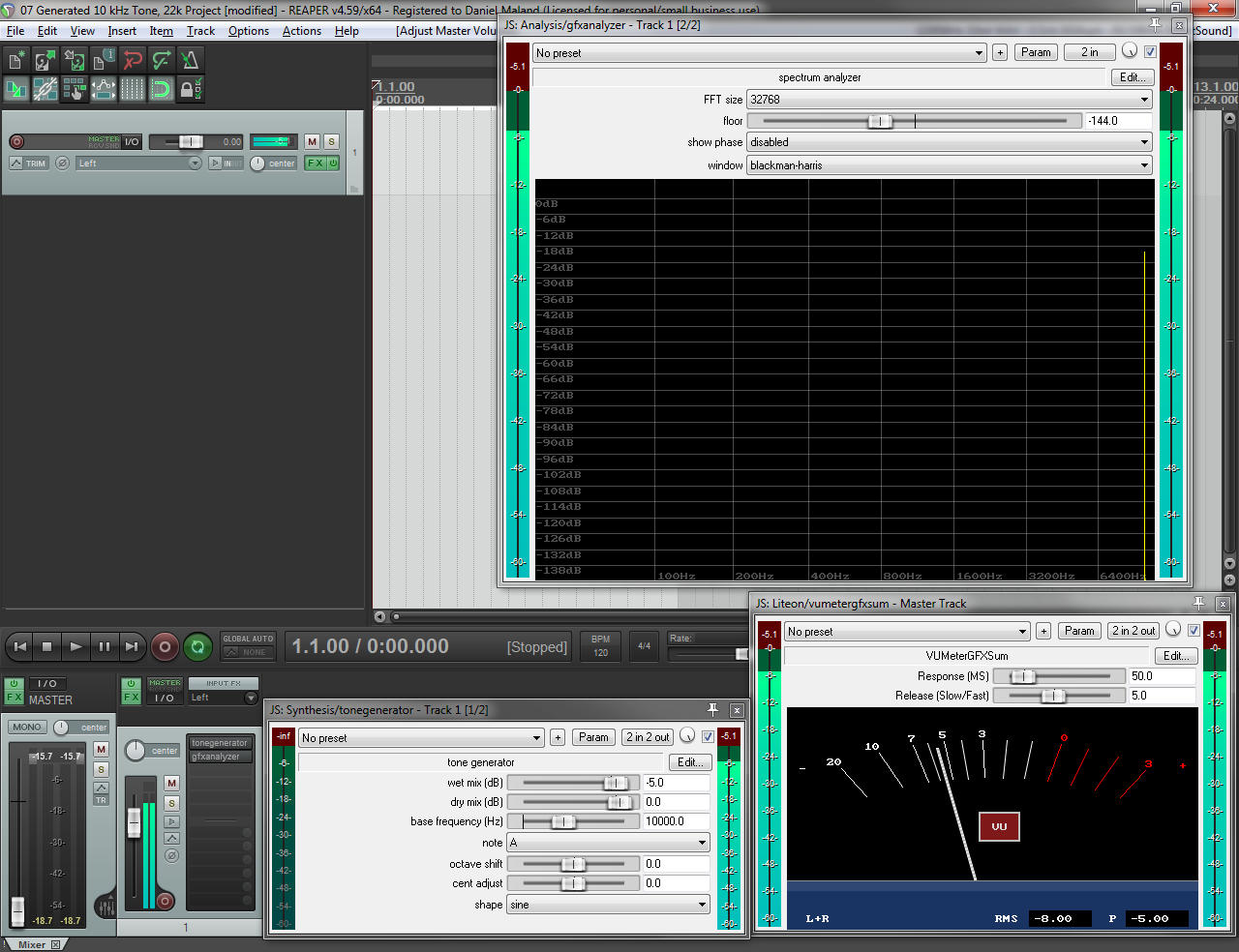
Conclusion: Hypothesis 2 is correct. At 22,500 samples per second, any given cycle of a 10 kHz wave only has two samples available to represent the signal. At 44.1 kHz sampling, any given cycle still only has four samples assigned. Event at 96 kHz, a 10 kHz wave has less than 10 samples assigned to it. If digital audio were an explicit representation of the wave, then such small numbers of samples being used to represent a signal should result in artifacts that are obvious either to the ear or to an analyzer. Any such artifacts are not observable via the above experiments, at any of the sampling rates used. The inference from this observation is that digital audio is an implicit representation of the signals being stored, and that sample rate does not affect the ability to accurately store information – as long as that information can be captured and stored at the sample rate in the first place.

Does A Higher Sample Rate Render Complex Material More Accurately?

Some people take major issue with the above experiment, because musical signals are not “naked” sine waves. Thus, we need an experiment which addresses the question of whether or not complex signals are represented more accurately by higher sample rates.

Hypothesis 1: A higher sampling rate does create a more faithful representation of complex waves, because complex waves are more difficult to represent than sine waves.

Hypothesis 2: A higher sampling rate does not create a more faithful representation of complex waves, because any complex wave is simply a number of sine waves modulating each other to varying degrees.

This test opens with the “08” project, which generates a complex sound at a 96 kHz sample rate. To make any artifacts easy to hear, the sound still uses pure tones, but the tones are spread out across the audible spectrum. Accordingly, the analyzer shows us 11 tones that read as “pure,” within experimental error. (Lower frequencies are less accurately depicted by the analyzer than high frequencies.)

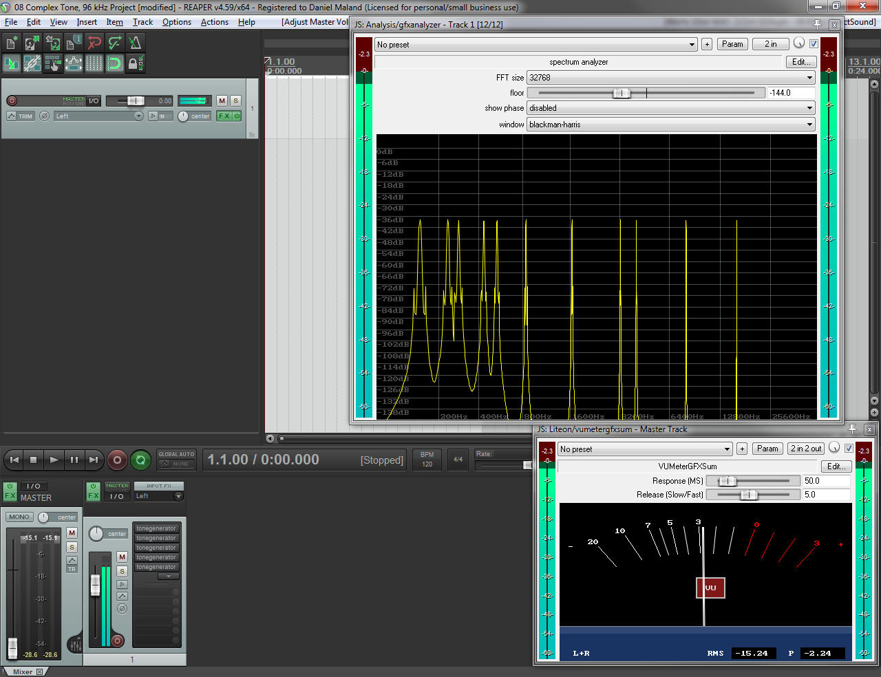
If we now load project “09,” we get a tone which is audibly and visibly the same, even though the project is now restricted to 44.1 kHz sampling. Although the analyzer’s trace has shifted to the right, we can still easily see 11, “pure” tones, free of artifacts beyond experimental error.

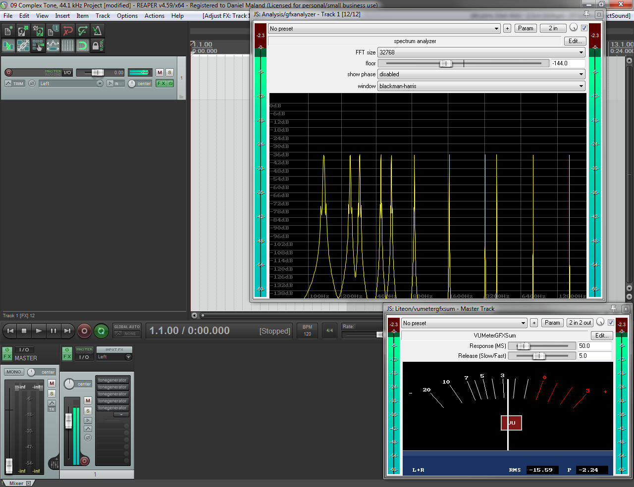
Conclusion: Hypothesis 2 is correct. A complex signal was observed as being faithfully reproduced, even with half the sampling data being available. An inference that can be made from this observation is that, as long as the highest frequency in a signal can be faithfully represented by a sampling rate, any additional material of lower frequency can be represented with the same degree of faithfulness.

Do Higher Bit Depths Better Represent A Given Signal, Independent Of Noise?

This question is at the heart of current debates about bit depth in consumer formats. The issue is whether or not larger bit-depths (and the consequentially larger file sizes) result in greater signal fidelity. This question is made more difficult because lower bit depths inevitably result in more noise. The presence of increasing noise makes a partial answer possible without experimentation: Yes, greater fidelity is afforded by higher bit-depth, because the noise level related to quantization error is inversely proportional to the number of bits available for quantization. The real question that remains is whether or not the signal, independent of the quantization noise, is more faithfully represented by having more bits available to assign sample values to.

Hypothesis 1: If noise is ignored, greater bit-depth results in greater accuracy. Again, the assumption is that digital is an explicit representation of the source material, and so more possible values per unit of voltage or pressure are advantageous.

Hypothesis 2: If noise is ignored, greater bit-depth does not result in greater accuracy. As before, the assumption is that we are using data in an implicit way, so as to reconstruct a signal at the output (and not directly represent it).

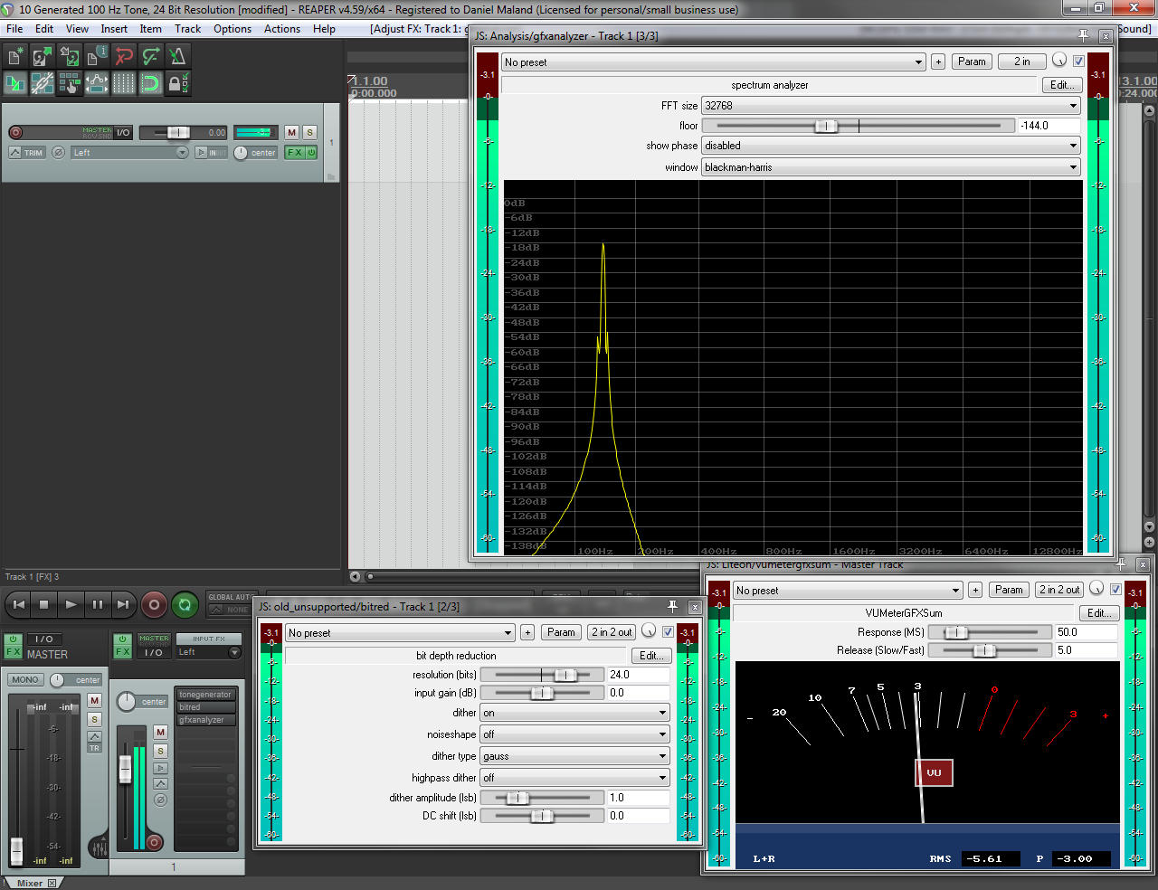
For this test, a 100 Hz tone was chosen. The reasoning behind this was because, at a constant 44.1 kHz sample rate, a single cycle of a 100 Hz tone has 441 sample values assigned to it. This relatively high number of sample positions should ensure that sample rate is not a factor in the signal being well represented, and so the accuracy of each sample value should be much closer to being an isolated variable in the experiment.

Project “10” generates a 100 Hz tone, with 24 bits of resolution. Dither is applied. Within experimental error, the tone appears “pure” on the analyzer. Any noise is below the measurement floor of -144 dBFS. (This measurement floor is convenient, because any real chance of hearing the noise would require listening at a level where the tone was producing 144 dB SPL, which is above the threshold of pain for humans.)

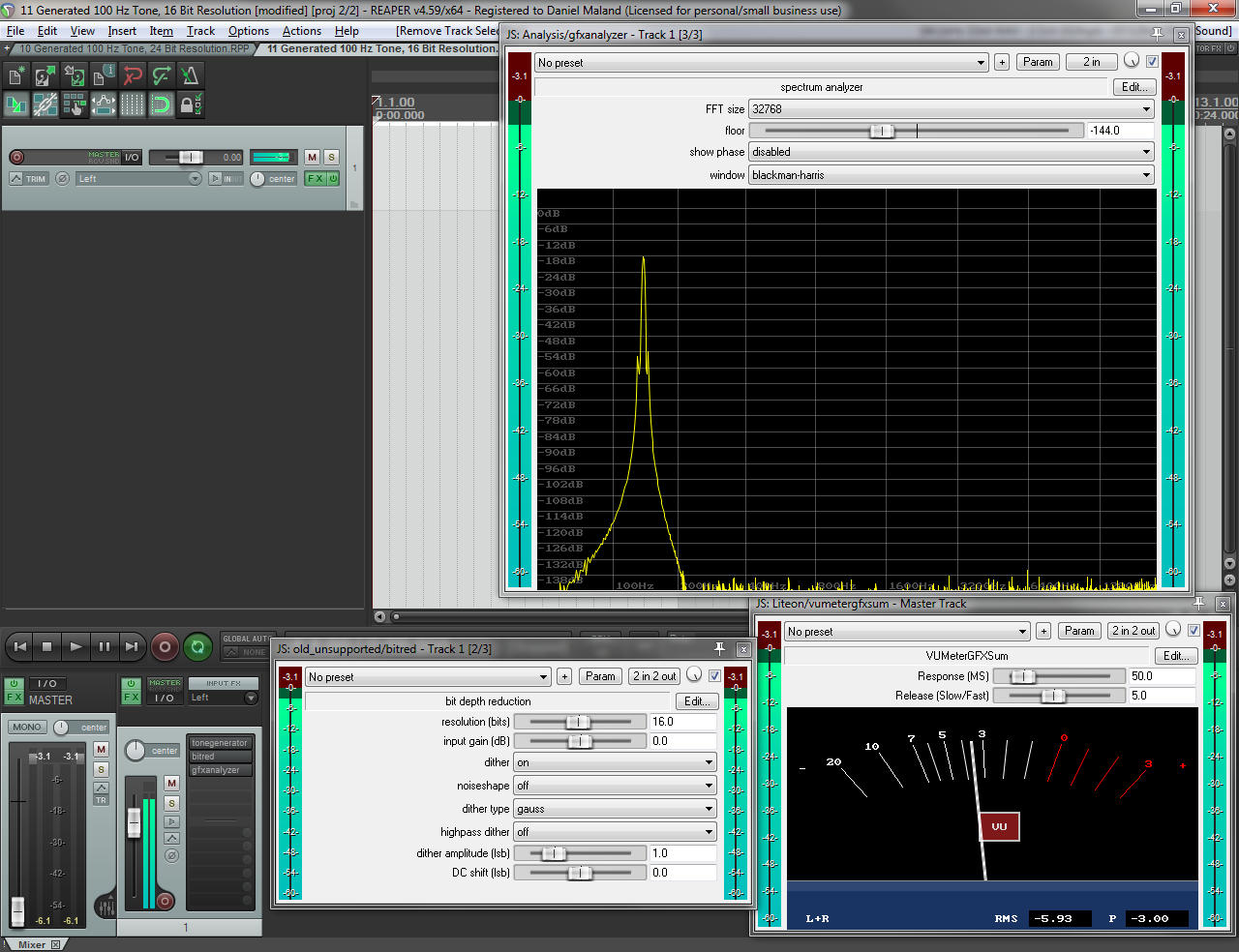
Project “11” generates the same tone, but at 16-bits. Noise is visible on the analyzer, but is inaudible when listening. No obvious harmonics or undertones are visible on the analyzer or audible to an observer.

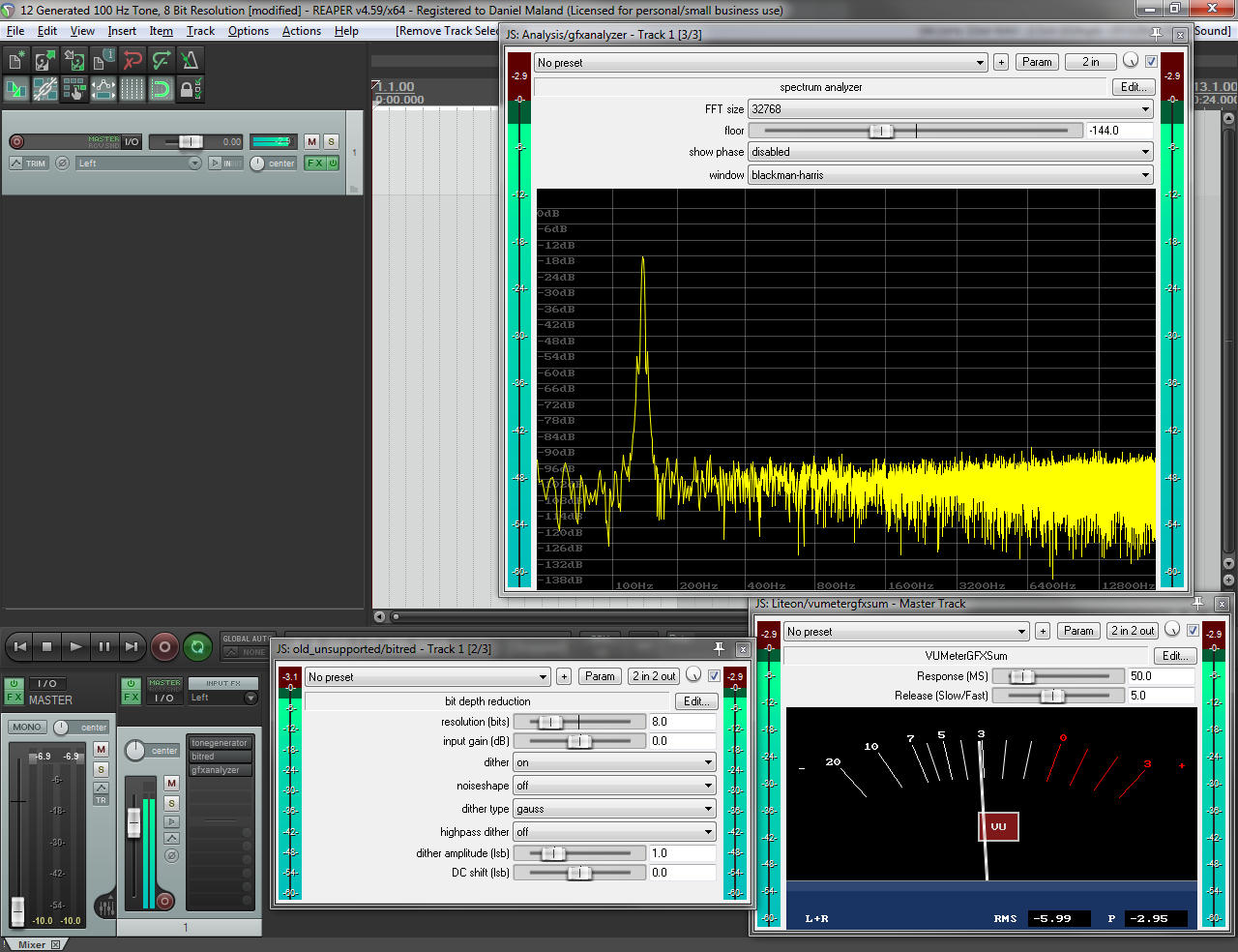
Project “12” restricts the signal to an 8-bit sample word. Noise is clearly visible on the analyzer, and easily audible to an observer. There are still no obvious harmonics or undertones.

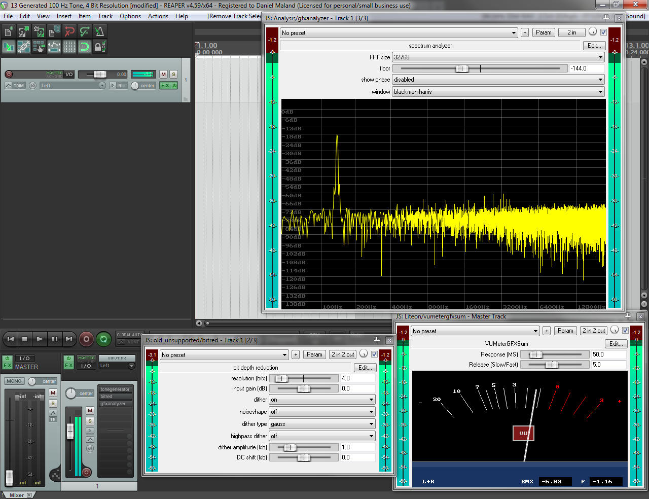
Project “13” offers only 4 bits of resolution. The noise is very prominent. The analyzer displays “spikes” which seem to suggest some kind of distortion, and an observer may hear something that sounds like harmonic distortion.

Conclusion: Hypothesis 2 is partially correct and partially incorrect (but only in a functional sense). For bit depths likely to be encountered by most listeners, a greater number of possible sample values does not produce demonstrably less distortion when noise is ignored. A pure tone remains observationally pure, and perfectly represented. However, it is important to note that, at some point, the harmonic distortion caused by quantization error appears to be able to “defeat” the applied dither. Even so, the original tone does not become “stair-stepped” or “rough.” It does, however, have unwanted tones superimposed upon it.