Tag Archives: Math

Gain Filtering

Full-bandwidth processing of audio levels can be neatly represented with graphs.

Please Remember:

The opinions expressed are mine only. These opinions do not necessarily reflect anybody else’s opinions. I do not own, operate, manage, or represent any band, venue, or company that I talk about, unless explicitly noted.

gainfilteringWant to use this image for something else? Great! Click it for the link to a high-res or resolution-independent version.

I really like cross-disciplinary concepts. The idea that fractal geometries are present in audio, for instance, is fascinating to me.

A non-audio discipline that I love very much is computer graphics. I’ve been a fan for a long time, long enough that I’ve been dinking around with pixels for (probably) longer than I’ve been dinking around with sound. A lot of sonic concepts are applicable in the visual world, and I even wrote a whole article about how audio processing can be understood in terms of graphics. In a certain sense, this article is a specialized extension of the other article I just mentioned.

A graphics program that I particularly enjoy is Vue. Vue is a “digital nature” program; a software package primarily meant for creating artificial environments. Whether you dig deeply into Vue or not, a concept and tool that you encounter fairly swiftly is that of filtering. Vue filters are a way of mapping input values to output values such that the correspondence isn’t necessarily 1:1. Vue lets you implement filters in various ways, but a full-control filter is represented as a graph:

vuefilter

Simple Gain Operations

Where things get interesting is when you come to a realization: That variable mapping of input levels to output levels is a “gain” operation, and that, of course, we have LOTS of gain operations in audio. What I mean is that audio-humans spend their entire careers applying signal-level multipliers to inputs. That multiplier might be “1,” also known as the multiplicative identity, which is the equivalent of passing an entire signal across a gain stage without changing it at all. That multiplier might also be “0,” which is what functionally occurs when you yank a fader down to -∞. Any signal level multiplied by zero becomes zero, so no signal appears at the gain stage output.

I’ll show you.

Here’s a Vue altitude function with a “straight through” filter. This is the equivalent of a fader being set to 0 dB. The difference between the input and the output is 0 dB – the gain multiplier is “1.”

1to1

Pulling a fader down results (or should result) in a signal transfer that is still linear, but also where an input of “i greater than 0” is output as “signal less than i.” In other words, a signal with a value greater than zero comes out as a version of itself with reduced level. Zero stays zero, because you can’t make actual silence quieter. Signals at low level disappear into the noise floor.

Important: Vue is meant to help you make things which look nice, so it’s not a model of a perfect audio circuit. As such, you’ll notice that the transfer of this “fader” is not entirely linear. This is a limitation of the example and not necessarily how you should expect things to work in real life.

faderdown

faderdownoutput

Slam the fader all the way down, and of course, nothing comes out. All signal levels map to zero.

faderfulldown

(I don’t really need to show a picture which is nothing but full-black pixels, do I?)

Dynamics Processing

Gain filtering is much more than simple faders, of course. Audio humans are very fond of non-linear gain operations, like compression.

Also Important: Vue filters are invariant with respect to time – they do not require even a nanosecond to react to an input signal. Almost every audio-oriented, nonlinear gain filter IS time variant in some respect. The delay between one gain state and another may be very small, and may only be required for gain which is returning to a multiplier of “1,” but the time involved still is NOT zero.

Anyway.

We’ll start with this unfiltered “signal:”

unfiltered

Dynamics Reduction

A basic compressor is a nonlinear gain filter that uses a breakpoint to join two linear gain functions with different slopes. The breakpoint is where the filter slope changes to resist signal level increases. In the parlance of sound practitioners, the breakpoint is the threshold. The slope of the post-breakpoint filter is the ratio.

compressor

compressed

A brickwall limiter is the same thing, but the post-breakpoint slope is horizontal (or very nearly so). Past the threshold, the output signal level does not increase appreciably, even if the input signal is large.

brickwall

brickwalled

A compressor with a “knee” is where the transition between gain slopes is, itself, sloped or curved. The compressor effectively incorporates multiple ratios, and if the “knee” covers a wide range of input levels, the entire compressor may appear to be nonlinear.

knee

kneed

Dynamics Expansion

A simple, downward expander is a kind of inverted compressor. It also features a breakpoint which joins two gain functions with different slopes. In an expander, however, the “compression” slope occurs before the breakpoint. Depending upon how you interpret the operation, an expansion device either pulls pre-breakpoint inputs down closer to silence, or you might say that it resists output increases until a certain input-side signal level is detected. (Things become even more interesting when you can supply inputs to the detector that are independent of the gain filter’s audible signal path.) The expander becomes 1:1 after the threshold. Fiddling with attack and release times may be required to make the transition pleasant, because the transition can involve not only an abrupt change in gain slope, but also a very high gain slope within that transition.

The possibility also exists to make the transition slope gradual, independent of the time required for a gain change to occur. In any case, here’s the simplified example:

expander

expanded

Gates are the “brickwall limiter” version of an expander. The gain filter applied to any signal below the threshold is “multiply by zero.”

gate

gated


The point of all this is to have an alternate route to interpreting how gain processing works. Maybe this is helpful; hopefully, it’s at least not confusing. Obviously, I can’t cover every quirk of every dynamics processor available, but maybe this helps you connect a few things in your mind.


Infinite Impulse Response

Coupled with being giant, resonant, acoustical circuits, PA systems are also IIR filters.

Please Remember:

The opinions expressed are mine only. These opinions do not necessarily reflect anybody else’s opinions. I do not own, operate, manage, or represent any band, venue, or company that I talk about, unless explicitly noted.

iirWant to use this image for something else? Great! Click it for the link to a high-res or resolution-independent version.

I’ve previously written about how impedance reveals the fabric of the universe. I’ve also written about how PA systems are enormous, tuned circuits implemented in the acoustic domain.

What I haven’t really gotten into is the whole concept of finite versus infinite impulse response. This follows along with the whole “resonant circuit” thing. A resonant circuit useful for audio incorporates some kind of feedback into its design, whether that design is intentional (an equalizer) or accidental (a PA system). Any PA system that amplifies the signals from microphones through loudspeakers which are audible to those same microphones is an IIR filter. That re-entrant sound is the feedback, even if the end result isn’t “feedback” in the traditional, loud, and annoying sense. Even if the PA system uses FIR filters for certain processing needs, the device as a whole exhibits infinite impulse response when viewed mathematically.

What the heck am I talking about?

FIR, IIR

Let’s first consider the key adjectives in the terms we’re using: “Finite” is one, and “infinite” is the other. The meanings aren’t complicated. Something that’s finite has an endpoint, and something that’s infinite does not. The infinite thingamabob just goes on forever.

The next bit to look at is the common subject that our adjectives are modifying. The impulse response of a PA system is what output the system produces when an input signal is applied.

So, if you stick both concepts together, a finite impulse response would mean that the PA system output relative to the input comes to a stop at some point. An infinite impulse response implies that our big stack of sound gear never comes to a stop relative to the input.

At this point, you’re probably thinking that I’ve got myself completely backwards. Isn’t a PA an FIR device? If we don’t have “classic” feedback, doesn’t the system come to a stop after a signal is removed? Well, no – not in the mathematical sense.

Functionally FIR, Mathematically IIR

First, let me talk about a clear exception. It’s entirely possible to use an assemblage of gear that’s recognizable as a PA system in a “playback only” context. The system is used to deliver sound to an audience, but there are no microphones involved in the realtime activity. They’re all muted, or not even present. Plug in any sort of signal source that is essentially impervious to sound pressure waves under normal operation, like a digital media player, and yes: You have a system that exhibits finite impulse response. The signal exiting the loudspeakers is never reintroduced to an input, so there’s no feedback. When the signal stops, the system (if you subtract the inherent, electronic noise floor) settles to a zero point.

But let’s look at some raw math when microphones are involved.

An acoustical signal is presented to a microphone capsule. The microphone converts the acoustical signal to an electrical one, and that electrical signal is then passed on to a whole stack of electronic doodads. The resulting electrical output is handed off to a loudspeaker, and the loudspeaker proceeds to convert the electrical signal into an acoustical signal. Some portion of that acoustical signal is presented to the same microphone capsule.

There’s our feedback loop, right?

Now, in a system that’s been tuned so as to behave itself, the effective gain on a signal traveling through the loop is a multiplier of less than one. (Converted into decibels, that means a gain of less than 0 dB.) Let’s say that the effective gain on the apparent pressure – NOT power – of a signal traversing our loop is 0.3. This means that our microphone “hears” the signal exiting the PA at a level that’s a bit more than 10 dB down from what originally entered the capsule.

If we start with an input sound having an apparent pressure of “1”:

Loop 1 apparent pressure = 0.3 (-10.5 dB)
Loop 2 apparent pressure = 0.09 (-21 dB)
Loop 3 apparent pressure = 0.027 (-31 dB)

Loop 10 apparent pressure = 0.0000059049 (-105 dB)

Loop 100 apparent pressure = 5.15e-53 (-1046 dB)

And so on.

In a mathematical sense, the PA system NEVER STOPS RINGING. (Well, until we hit the appropriate mute button or shut off the power.) The apparent pressure never reaches zero, although it gets very close to zero as time goes on.

And again, this brings us back to the concept of our rig being functionally FIR, even though it’s actually IIR. It is entirely true that, at some point, the decaying signal becomes completely swallowed up in both the acoustical and electrical noise floors. After a number of rounds through the loop, the signal would not be large enough to meaningfully drive an output transducer. As far as humans are concerned, the timescale required for our IIR system to SEEM like an FIR system is small.

Fair enough – but don’t lose your sense of wonder.

Fractal Geometries and Application

Although the behavior of a live-audio rig might not quite fit the strict definition of what mathematicians call an iterated function system, I would argue that – intriguingly – a PA system’s IIR behavior is fractal in nature. The number of loop traversals is infinite, although we may not be able to perceive those traversals after a certain number of iterations. Each traversal of the loop transforms the input in a way which is ultimately self-similar to all previous loop inputs. A large peak may develop in the frequency response, but that peak is a predictable derivation of the original signal, based on the transfer function of the loop. Further, in a sound system that has been set up to be useful, the overall result is “contractive:” The signal’s deviation from silence becomes smaller and smaller, and thus the signal peaks come closer and closer together.

I really do think that the impulse behavior of a concert rig might not be so different from a fractal picture like this:

sonicbutterful

And at the risk of an abrupt stop, I think there’s a practical idea we can derive from this whole discussion.

A system may be IIR in nature, but appear to be FIR after a certain time under normal operating conditions. If so, the transition time to the apparent FIR endpoint should be small enough that the system “ring time” does not perceptibly add to the acoustical environment’s reverb time.

Think about it.


How Much Output Should I Expect?

A calculator for figuring out how much SPL a reasonably-powered rig can develop.

Please Remember:

The opinions expressed are mine only. These opinions do not necessarily reflect anybody else’s opinions. I do not own, operate, manage, or represent any band, venue, or company that I talk about, unless explicitly noted.

howloudWant to use this image for something else? Great! Click it for the link to a high-res or resolution-independent version.

As a follow-on to my article about buying amplifiers, I thought it would be helpful to supply an extra tool. The purpose of this calculator is to give you an idea of the SPL delivered by a “sanely” powered audio rig.

A common mistake made when estimating output is to assume that the continuous power the amp is rated for will be easily applied to a loudspeaker. This leads to inflated estimations of PA performance, because, in reality, actually applying the rated continuous power of the amp is relatively difficult. It’s possible with a signal of narrow bandwidth and narrow dynamic range – like feedback, or sine-wave synth sounds, but most music doesn’t behave that way. Most of the time, the signal peaks are far above the continuous level…

…and, to be brutally honest, continuous output is what really counts.


This Calculator Requires Javascript

This calculator is an “aid” only. You should not rely upon it solely, especially if you are using it to help make decisions that have legal implications or involve large amounts of money. (I’ve checked it for glaring errors, but other bugs may remain.) The calculator assumes that you have the knowledge necessary to connect loudspeakers to amplifiers in such a way that the recommended power is applied.


Enter the sensitivity (SPL @ 1 watt @ 1 meter) of the loudspeakers you wish to use:

Enter the peak power rating of your speakers, if you want slightly higher performance at the expense of some safety. If you prefer greater safety, enter half the peak rating:

Enter the number of loudspeakers you intend to use:

Enter the distance from the loudspeakers to where you will be listening. Indicate whether the measurement is in feet or meters. (Measurements working out to be less than 1 meter will be clamped to 1 meter.)

Click the button to process the above information:

Recommended amplifier continuous power rating at loudspeaker impedance:
0 Watts

Calculated actual continuous power easily deliverable to each loudspeaker:
0 Watts

Calculated maximum continuous output for one loudspeaker at 1 meter:
0 dB SPL

Calculated maximum continuous output for one loudspeaker at the given listening position:
0 dB SPL

Calculated maximum continous output for entire system at the given listening position:
0 dB SPL

How The Calculator Works

First, if you want to examine the calculator’s code, you can get it here: Maxoutput.js

This calculator is intentionally designed to give a “lowball” estimate of your total output.

First, the calculator divides your given amplifier rating in half, operating on the assumption that an amp rated with sine-wave input will have a continuous power of roughly half its peak capability. An amp driven into distortion or limiting will have a higher continuous output capability, although the peak output will remain fixed.

The calculator then assumes that it will only be easy for you to drive the amp to a continuous output of -12 dB referenced to the peak output. Driving the amp into distortion or limiting, or driving the amp with heavily compressed material can cause the achievable continuous output to rise.

The calculator takes the above two assumptions and figures the continuous acoustic output of one loudspeaker with a continuous input of -12 dB referenced to the peak wattage available.

The next step is to figure the apparent level drop due to distance. The calculator uses the “worst case scenario” of inverse square, or 6 dB of SPL lost for every doubling of distance. This essentially presumes that the system is being run in an anechoic environment, where sound pressure waves traveling away from the listener are lost forever. This is rarely true, especially indoors, but it’s better to return a more conservative answer than an “overhyped” number.

The final bit is to sum the SPLs of all the loudspeakers specified to be in the system. This is tricky, because the exact deployment of the rig has a large effect – and the calculator can’t know what you’re going to do. The assumption is that all the loudspeakers are audible to the listener, but that half of them appear to be half as loud.


How Powerful An Amp Should I Buy?

For safety, match the continuous ratings. For performance, match the peak ratings.

Please Remember:

The opinions expressed are mine only. These opinions do not necessarily reflect anybody else’s opinions. I do not own, operate, manage, or represent any band, venue, or company that I talk about, unless explicitly noted.

gx5Want to use this image for something else? Great! Click it for the link to a high-res or resolution-independent version.

For people who buy passive speakers (loudspeakers driven by amplifiers in separate enclosures), the question of how much amp to purchase is somewhat sticky. Ask it, and you’ll get all manner of advice. Some of it good, some of it bad, and some of it downright ludicrous. You’re very likely to hear a bunch of hoo-ha about how using too small of an amp is dangerous (it isn’t), because clipping kills drivers (it doesn’t). Someone will eventually say that huge amps give you more headroom (sorry, but no). All kinds of “multipliers” will be bandied about.

You may become more confused than when you started.

In my opinion, the basic answer is pretty simple, although the explanation will take a bit of time:

First, note that even though physicists will tell you that there’s no such thing as “RMS power,” there IS such a thing as the average or continuous power derived from a certain RMS voltage input. That’s what “RMS power” on a spec sheet means.

For a reasonable balance of safety and performance, match the amp’s continuous rating with the loudspeaker’s continuous rating.

(If you cannot find a loudspeaker’s continuous rating, clearly stated, on a spec sheet, take the smallest rating you can find and divide by two. If you cannot easily find an amp’s continuous rating on a spec sheet, just choose a different amplifier.)

For slightly more performance at the cost of some safety, choose an amplifier with a continuous rating that is half the peak power handling of the loudspeaker.

Depending upon how a loudspeaker is rated, the “safety” and “performance” criteria may actually end up giving you the same answer. This is perfectly acceptable.

Now then. Here’s how I justify my advice.

Peak / √2

The first step here is to understand a bit more about some basic bath and science regarding amplifiers.

A power amplifier is really a voltage amplifier that can deliver enough current to drive a loudspeaker motor. A power amplifier has an upper limit to how much voltage it can develop, as you might expect. That maximum voltage, combined with the connected load and the amplifier’s ability to supply current, determines the amplifier’s peak power.

In normative cases, an amplifier’s peak output is an “instantaneous” event. If the amplifier is contributing no noticeable distortion to the signal, then the signal “swing” is reaching the amplifier’s maximum voltage for a very small amount of time. (Ideally, an infinitely small duration.) Again, if we assume normal operation, an amplifier spends the overwhelming majority of its life producing less than maximum output.

An amplifier’s continuous power, on the other hand, is an average over a significant amount of time. This is why engineers say things like “power is the area under the curve.” An undistorted peak with nothing before or after it has virtually no area under the curve, whereas a signal that never gets anywhere near peak output (but lasts for several seconds) can have very significant area under the curve.

For audio voltages, we use RMS averaging. One important reason for this is because audio voltages corresponding to sound-pressure events have positive and negative swing. For, say, one cycle of a sine wave, the arithmetic mean would be zero – the wave has equal positive and negative value. RMS averaging, on the other hand, squares each input value. As such, positive values remain positive, and negative values become positive (-2 squared, for instance, is 4).

In the case of an undistorted sine wave, the RMS voltage is the peak voltage divided by √2, or about 1.414.

Here’s a graph to make this all easier to visualize. This is a plot of a very small, hypothetical power amplifier passing an undistorted sine wave. The maximum output voltage is ± 2 volts. That means that the RMS voltage is 2/√2, or 1.414.

2sinx

Here’s where the rubber begins to meet the road. Let’s assume that this amplifier is mated to a loudspeaker with an impedance of 8 Ohms.

Power = Voltage Squared / Resistance

Peak Power = Peak Voltage Squared / Resistance

Continuous Power = RMS Voltage Squared / Resistance

Peak Power = 2^2 / 8 = 0.5 Watts

Continuous Power = (2 / √2)^2 / 8 = 0.25 watts

For a sine wave, the continuous power is half the peak power, or 3 dB down. This is the main justification for the above statement: “For slightly more performance at the cost of some safety, choose an amplifier with a continuous rating that is half the peak power handling of the loudspeaker.” Assuming that the amplifier was rated using sine-wave input (a reasonable assumption at the time of this writing), the peak output of the amplifier will be twice the continuous rating, and therefore match up with the peak power handling of the loudspeaker. By the same token, the “safety” recommendation means that the peak amp output will be either at or far below the peak rating of the loudspeaker – especially since many loudspeakers are claimed to handle peaks that are four times greater than the recommended continuous input.

An amplifier with peak output capabilities that exceeds the peak handling capabilities of a loudspeaker is a liability, not an asset. In live-sound, all kinds of mishaps can occur which will drive an amp all the way to its maximum output. If that maximum output is too high, you might just have an expensive repair on your hands. If the maximum amplifier output plays nicely with the loudspeaker’s capabilities, however, accidents are much less worrisome.

So, there’s the explanation in terms of peak power. What about some other angles?

A More Holistic Picture

Musical signals running through a PA are usually not pure sine waves. They can be decomposed into pure tones, certainly, but the total signal behavior is not “RMS voltage = peak / √2.” You might have an overall continuous power level that’s 10 dB, 12 dB, 15 dB, or even farther down from the peaks. Why could you still run into problems?

The short answer is that not all drivers are created equally, and EQ can make them even more unequal. Further, EQ can cause you to be rather more unkind than you might realize.

For a bit more detail, let’s make up a compromise example using pink noise that has a crest factor of slightly more than 13 decibels. If we run the signal full-range, we get statistics that look like this:

fullrangepink

Let’s say that we have a QSC GX5 plugged into an 8 Ohm loudspeaker. A GX5 is rated for 500 watts continuous into that load, so a reasonable guess at peak output is 1000 watts. To find -13 dB in terms of power:

10 log (x / 1000) = -13 dB

log (x / 1000) = -1.3 dB

10^-1.3 = 0.0501 = x / 1000

x = 50 watts

(Of course, -13 dB can also be found by dividing -10 dB, or 0.1 X power, by two.)

That power hits a passive crossover, which splits the full range signal into appropriate passbands for the various drivers. In an affordable, two-way box, the crossover might be something like 12 dB / octave at 2000 Hz. If I filter the noise accordingly, I get this for what the LF driver “sees”:

lfpink

Compared to the original peak, the LF driver is seeing about -14.5 dB continuous, or a bit more than 35 watts. Some instantaneous levels of about 800 watts come through, but the driver can probably soak those up if most of the energy is above, say, 40 Hz.

For the HF driver:

hfpink

Again, we have to compare things to the original peak of -0.89 dB, so the continuous measurement is actually 17.8 dB down from there. Also, an additional complication exists. The HF driver is probably padded down at the crossover, because a compression driver mated to a horn can have a sensitivity of 104+ dB @ 1 watt @ 1 meter, whereas the cone driver might be only 96 dB or so. In the case of an 8 dB pad, the total continuous power being experienced by the HF portion of the box could reasonably be said to be -25.8 dB from the peak power. That’s something like 2.5 watts, with peaks at 37 watts or so.

No problem, right?

But what if you bought a really powerful amp – like one that could deliver peaks of 2000 watts?

Your HF driver would still be okay, but your LF driver might not be. Sure, 70 watts continuous wouldn’t burn up the voice coil, but what would 1600 watt peaks do? Especially if the information is “down deep,” that poor cone is likely to get ripped apart. If somebody does something like dropping a mic…well…

And what if someone applies the dreaded “smiley face” EQ, and then drives the amp right up to the clip lights?

At first, things still look OK. The continuous signal is still 13 dB down from the peaks.

smileyeq

The LF driver is getting something like this:

smileylf

For the reasonably-sized amp, the LF peaks are at 0.7 dB below clipping, or 850 watts. That’s probably a little too much for the driver, but it might not die immediately – unless a huge impulse under 40 Hz comes through. With the oversized amplifier, you now have 1700 watt peaks, which are beating up your LF cone just that much faster.

In the world of the HF driver:

smileyhf

Using the appropriate amp, the HF driver isn’t getting cooked at all. In fact, the abundance of LF content actually pushes the continuous and peak power down slightly. Even the big amp isn’t an issue.

Of course, someone could decide to only crank the highs, because they want “that crispness, you know?” (This would also correspond to program material that’s heavily biased towards HF information.)

crispy

Now things get a little scary. Scale the measurement right up to clipping (0 dB, because this reading was taken “in isolation”), and the peaks are padded down to only -8 dB. That’s almost 160 watts, which is beyond the peak tolerance of the driver. The 13 watts of continuous input isn’t hurting anything, but the poor little HF unit is taking plenty of abuse.

Connect the “more headroom, dude!” amplifier, and it gets much worse. One 320 watt peak will surely be enough to end the life of the unit, and if (by some miracle) the peaks are limited but the continuous power isn’t…well, the driver might withstand 26 watts continuous, but just two more dB and you get 41 watts. The poor baby is probably roasting, if it’s an affordable unit.

Conclusions

I’m sorry if all that caused your eyes to glaze over. Here’s how it shakes out:

An amp which has a continuous rating that matches the loudspeaker’s continuous rating does a lot to protect you from abuse, accidents, and stupidity. Using an amplifier that has a peak rating equal to the speaker’s peak rating lets you get a bit more level (3 dB) while still shielding you from a lot of problems. You can still get yourself into trouble, but it takes some effort.

Running an amplifier which goes a long way past the peak rating of a speaker enclosure is just asking for something to get wrecked. Yes, you can make it all work if you’re careful and use well-set processing to keep things sane – but that’s beyond the scope of this article.

If a conservatively powered PA doesn’t get loud enough for you, you need more PA. That is, you need more boxes powered at the same per-box level, or boxes that are naturally louder, or boxes that will take more power.


Not Remotely Successful

Just getting remote access to a mix rig is not a guarantee of being able to do anything useful with that remote access.

Please Remember:

The opinions expressed are mine only. These opinions do not necessarily reflect anybody else’s opinions. I do not own, operate, manage, or represent any band, venue, or company that I talk about, unless explicitly noted.

sorrytabletsWant to use this image for something else? Great! Click it for the link to a high-res or resolution-independent version.

The nature of experimentation is that your trial may not get you the expected results. Just ask the rocket scientists of the mid-twentieth century. Quite a few of their flying machines didn’t fly. Some of them had parts that flew – but only because some other part exploded.

This last week, I attempted to implement a remote-control system for the mixing console at my regular gig. I didn’t get the results I wanted, but I learned a fair bit. In a sense, I think I can say that what I learned is more valuable than actually achieving success. It’s not that I wouldn’t have preferred to succeed, but the reality is that things were working just fine without any remote control being available. It would have been a nice bit of “gravy,” but it’s not like an ability to stride up to the stage and tune monitors from the deck is “mission critical.”

The Background

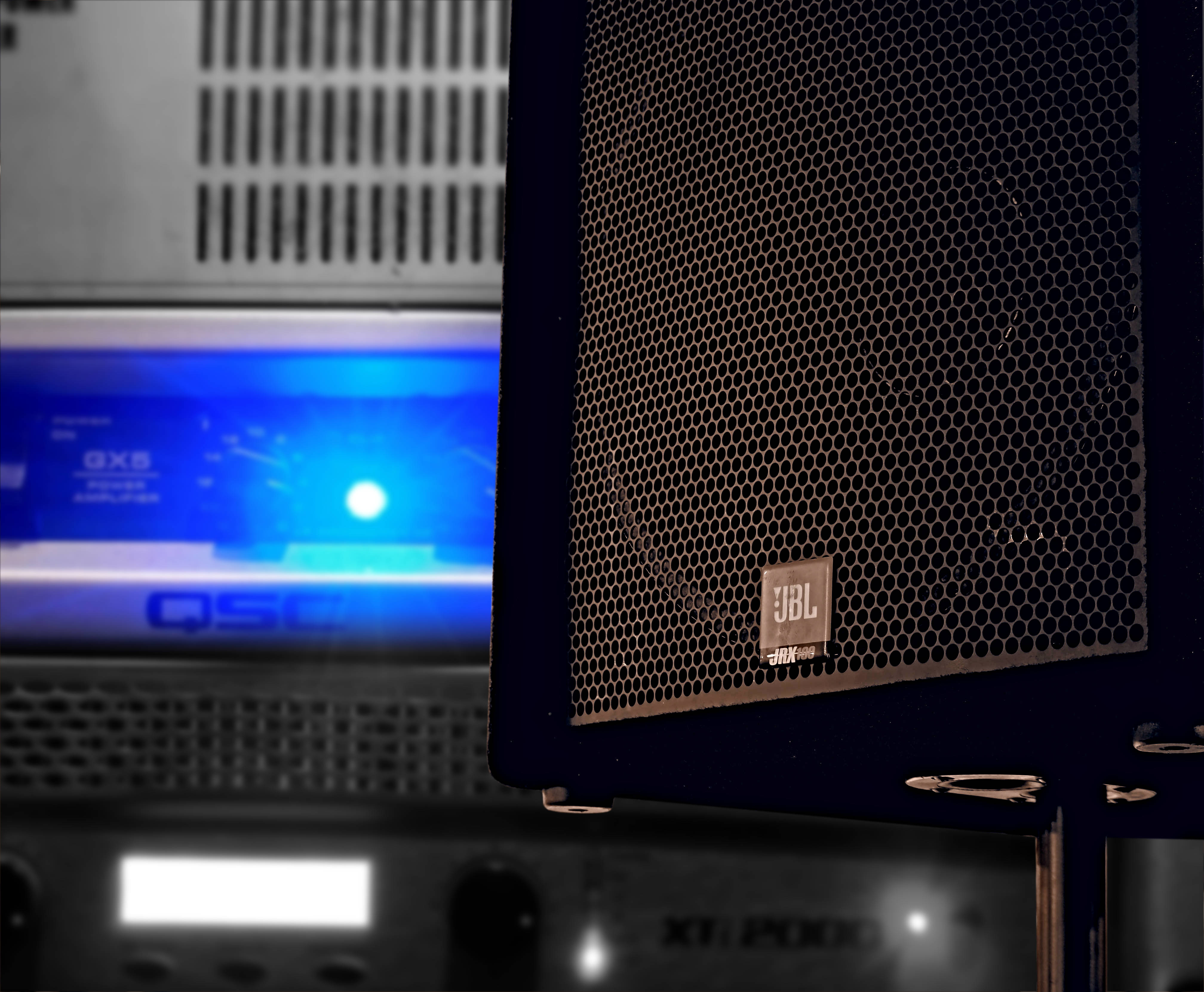
If you’re new to this site, you may not know about the mix rig that I use regularly. It’s a custom-built console that runs on general computing hardware. It started as a SAC build, but I switched to Reaper and have stayed there ever since.

To the extent that you’re talking about raw connectivity, a computer-hosted mix system is pre-primed for remote control. Any modern computer and accessible operating system will include facilities for “talking” to other devices over a network. Those connectivity facilities will be, at a basic level, easy to configure.

(It’s kind of an important thing these days, what with the Internet and all.)

So, when a local retailer was blowing out 10″ Android tablets for half price, I thought, “Why not?” I had already done some research and discovered that VNC apps could be had on Android devices, and I’ve set up VNC servers on computers before. (It’s not hard, especially now that the installers handle the network security configuration for you.) In my mind, I wasn’t trying to do anything exotic.

And I was right. Once I had a wireless network in place and all the necessary software installed, getting a remote connection to my console machine was as smooth as butter. Right there, on my tablet, was a view of my mixing console. I could navigate around the screen and click on things. It all looked very promising.

There’s a big difference between basic interaction and really being able to work, though. When it all came down to it, I couldn’t easily do the substantive tasks that would make having a remote a handy thing. It didn’t take me long to realize that tuning monitors while standing on the deck was not something I’d be able to do in a professional way.

A Gooey GUI Problem

At the practical level, the problem I was having was an interface mismatch. That is, while my tablet could display the console interface, the tablet’s input methodology wasn’t compatible with the interface being displayed.

Now, what the heck does that mean?

Reaper (and lots of other audio-workstation interfaces) are built for high-precision pointing devices. You might not think of a mouse or trackball as “high precision,” but when you couple one of those input devices with the onscreen pointer, high precision is what you get. The business-end of the pointer is clearly visible, only a few pixels wide, and the “interactivity radius” of the pointer is only slightly larger. There is an immediately obvious and fine-grained discrimination between what the pointer is set to interact with, and what it isn’t. With this being the case, the software interface can use lots of small controls that are tightly packed.

Additionally, high-precision pointing allows for fast navigation across lots of screen area. If you have the pointer in one area of the screen and invoke, say, an EQ window that pops open in another area, it’s not hard to get over to that EQ window. You flick the mouse, your eye finds the pointer, you correct on the fly, and you very quickly have control localized to the new window. (There’s also the whole bonus of being able to see the entire screen at once.) With high-precision input being available, the workstation software can make heavy use of many independent windows.

Lastly, mice and other high-precision pointers have buttons that are decoupled from the “pointing” action. Barring some sort of failure, these buttons are very unambiguous. When the button is pressed, it’s very definitely pressed. Clicks and button holds are sharply delineated and easily parsed by both the machine and the user. The computer gets an electrical signal, and the user gets tactile feedback in their fingers that correlates with an audible “click” from the button. This unambiguous button input means that the software can leverage all kinds of fine-grained interactions between the pointer position and the button states. One of the most important of those interactions is the dragging of controls like faders and knobs.

So far so good?

The problem starts when an interface expecting high-precision pointing is displayed on a device that only supports low-precision pointing. Devices like phones and tablets that are operated by touch are low-precision.

Have you noticed that user interfaces for touch-oriented devices are filled with big buttons, “modal” elements that take over the screen, and expectations for “big” gestures? It’s because touch control is coarse. Compared to the razor-sharp focus of a mouse-driven pointer, a finger is incredibly clumsy. Your hand and finger block a huge portion of the screen, and your finger pad contacts a MASSIVE area of the control surface. Sure, the tablet might translate that contact into a single-pixel position, but that’s not immediately apparent (or practically useful) to the operator. The software can’t present you with a bunch of small subwindows, as the miniscule interface elements can’t be managed easily by the user. In addition, the only way for the touch-enabled device to know the cursor’s location is for you to touch the screen…but touch, by necessity, has to double as a “click.” Interactions that deal with both clicks and movement have to be forgiving and loosely parsed as a result.

Tablets don’t show big, widely spaced controls in a single window because it looks cool. They do it because it’s practical. When a tablet displays a remote interface that’s made for a high-precision input methodology, life gets rather difficult:

“Oh, you want to display a 1600 x 900, 21″ screen interface on a 1024 X 600, 10″ screen? That’s cool, I’ll just scale it down for you. What do you mean you can’t interact with it meaningfully now?”

“Oh, you want to open the EQ plugin window on channel two? Here you go. You can’t see it? Just swipe over to it. What do you mean you don’t know where it is?”

“Oh, you want to increase the send level to mix three from channel four? Nice! Just click and drag on that little knob. That’s not what you touched. That’s also not what you touched. Try zooming in. I’m zoomi- wait, you just clicked the mute on channel five. Okay, the knob’s big now. Click and drag. Wait…was that a single click, or a click and hold? I think that was…no. Okay, now you’re dragging. Now you’ve stopped. What do you mean, you didn’t intend to stop? You lifted your finger up a little. Try again.”

With an interface mismatch, everything IS doable…but it’s also VERY slow, and excruciatingly difficult compared to just walking back to the main console and handling it with the mouse. Muting or unmuting a channel is easy enough, but mixing monitors (and fighting feedback) requires swift, smooth control over lots of precision elements. If the interface doesn’t allow for that, you’re out of luck.

Control States VS. Pictures Of Controls

So, can systems be successfully operated by remotes that don’t use the same input methodology as the native interface?

Of course! That’s why traditional-surface digital consoles can be run from tablets now. The tablet interfaces are purpose-built, and involve “state” information about the main console’s controls. My remote-control solution didn’t include any of that. The barrier for me is that I was trying to use a general-purpose solution: VNC.

With VNC, the data transmitted over the network is not the state of the console’s controls. The data is a picture of the console’s controls only, with no control-state data involved.

That might seem confusing. You might be saying, “But there is data about the state of the controls! You can see where the faders are, and whether the mutes are pressed, and so on.”

Here’s the thing, though. You’re able to determine the state of the controls because you can interpret the picture. That determination you’ve made, however, is a reconstruction. You, as a human, might be seeing a picture of a fader at a certain level. Because that picture has a meaning that you can extract via pattern recognition, you can conceptualize that the fader is in a certain state – the state of being at some arbitrary level of gain. To the computer, though, that picture has no meaning in terms of where that fader is.

When my tablet connects to the console via VNC, and I make the motions to change a control’s state, my tablet is NOT sending information to the console about the control I’m changing. The tablet is merely saying “click at this screen position.” For example, if clicking at that screen position causes a channel’s mute to toggle, that’s great – but the only machine aware of that mute, or whether that mute is engaged or disengaged, is the console itself. The tablet itself is unaware. It’s up to me to look at the updated picture and decide what it all means…and that’s assuming that I even get an updated picture.

The cure to all of this is to build a touch-friendly interface which is aware of the state of the controls being operated. You can present the knobs, faders, and switches in whatever way you want, because the remote-control information only concerns where that control should be set. The knobs and faders sit in the right place, because the local device knows where they are supposed to be in relation to their control state. Besides solving the “interface mismatch” problem, this can also be LIGHT YEARS more efficient.

(Disclaimer: I am not intimately aware of the inner workings of VNC or any console-remote protocol. What follows are only conjectures, but they seem to be reasonable to me.)

Sending a stream of HD (or near HD) screenshots across a network means quite a lot of data. If you’re using jpeg-esque compression, you can crush each image down to 100 kilobytes and still have things be usable. VNC can be pretty choosy about what it updates, so let’s say you only need one full image every second. You won’t see meters move smoothly or anything like that, but that’s the price for keeping things manageable. The data rate is about 819 kbits/ second, plus the networking overhead (packet headers and other communication).

Now then. Let’s say we’ve got some remote-control software that handles all “look and feel” on the local device (say, a tablet). If you represent a channel as an 8-bit identifier, that means you can have up to 256 channels represented. You don’t need to actually update each channel all the time to simply get control. Data can just be sent as needed, of course. However, if you want to update the channel meters 30 times per second, that meter data (which could be another 8-bit value) has to be attached to each channel ID. So, 30 times a second, 256 8-bit identifiers get 8-bits of meter information data attached to each of them. Sixteen bits multiplied by 256 channels, multiplied by 30 updates/ second works out to about 123 kbits/ second.

Someone should check my math and logic, but if I’m right, nicely fluid metering across a boatload of channels is possible at less than 1/6th the data rate of “send me a screenshot” remote control. You just have to let the remote device handle the graphics locally.

Control-state changes are even easier. A channel with fader, mute, solo, pan, polarity, a five-selection routing matrix, and 10 send controls needs to have 20 “control IDs” available. A measly little 5-bit number can handle that (and more). If the fader can handle 157 “integer” levels (+12 dB to -143 dB and “-infinity”) with 10 fractional levels of .1 dB between each integer (1570 values total), then the fader position can be more than adequately represented by an 11-bit number. If you touch a fader and the software sends a control update every 100th of a second, then a channel ID, control ID, and fader position have to be sent 100 times per second. That’s 24 bits multiplied by 100, or 2.4 kbits/ second.

That’s trivial compared to sending screenshots across the network, and still almost trivial when compared to the “not actually fast” data rate required to update the meters all the time.

Again, let me be clear. I don’t actually know if this is how “control state” remote operation works. I don’t know how focused the programmers are on network data efficiency, or even if this would be a practical implementation. It seems plausible to me, though.

I’m rambling at this point, so let me tie all this up: Remote control is nifty, and you can get the basic appearance of remote control with a general purpose solution like VNC. If you really need to get work done in a critical environment, though, you need a purpose built solution that “plays nice” at both the local and remote ends.


The Cost Effectiveness Of Premium Soda

$1.00 per usage cycle is a magical number.

Please Remember:

The opinions expressed are mine only. These opinions do not necessarily reflect anybody else’s opinions. I do not own, operate, manage, or represent any band, venue, or company that I talk about, unless explicitly noted.

1Want to use this image for something else? Great! Click it for the link to a high-res or resolution-independent version.

Whether or not you like them, energy drinks are actually pretty cheap.

That is to say, for about a buck you buy a can of soda. You consume the contents of that can and chuck out the container without a second thought. You got exactly one use out that product for $1.00, and you barely noticed the transaction at all.

In my mind, that’s a pretty strong definition of “cheap, and cost effective.” The acquisition price was basically forgettable on its own, and the amount of utility you got for that acquisition price was reasonable to you – maybe at an unconscious level, but reasonable.

For show-production techs, there comes a day when we either have to procure our own gear or procure gear with someone else’s money. On that day, we have to think about cost effectiveness. We may not give it the conscious thought it deserves, but some sort of mental evaluation takes place. In this business, an oft-occurring result of considering gear is “sticker shock.” We look at the price attached to something and go “Geeze! That’s a lot!” Sometimes the reaction is justified, but there are other times when the number associated with entry isn’t rationally compared with what happens after the entry occurs. In certain cases, the long-term utility of a piece of gear actually makes the entry cost seem microscopic – but that can be hard to see at the time.

Now, there are all kinds of ways to determine cost-effectiveness. Some available methods are incredibly granular, taking into account depreciation, cost of transport, industry acceptance, and so on. Dave Rat, for example, put together a rather interesting “Buy Vs. Lease” calculator that you can find at the bottom of this post. If you know me, you know that I’m a great appreciator of granularity. I like to be able to deal with all kinds of minutiae. I like sniper-rifle focus in lots of areas, especially when it comes to mixing FOH (Front Of House) and monitors from the same spot.

But when it comes to making purchasing decisions in a rational way, I think that getting buried in a barrage of detailed considerations can lead to paralysis. I think that a basic shorthand can help make cost-effectiveness decisions go much more quickly – which provides a shortcut to the fun part, which IS GETTING NEW GEAR AM I RIGHT?

Anyway.

When I talk about shorthand, I mean REALLY shorthand. It’s probably one of the quickest questions you can ask yourself about a piece of gear: “Will I be able to get enough usage out of this item that each deployment cycle will have cost $1.00 or less?”

Of Power Amps and Microphones

At my regular gig, the amplifier for the full-range FOH loudspeakers is a QSC GX5. It’s been very good to us, and by my shorthand test, it’s been entirely inexpensive.

See, I just passed my four-year mark at the job. We do just a bit more than 104 shows per year, so the amp has about 416 shows on it. GX5 amps retail for $400 when brand new. Divide $400 by 416 shows, and you get a “cost effectiveness factor” of $0.96/ deployment. To be brutally honest, that’s peanuts. It’s not that we’d want to, but at this point we could just give the amp away and have lost nothing more – proportionally speaking – than if someone had bought and consumed about 400 energy drinks.

And the amp is still going strong! (It needed a replacement power switch last weekend, but that’s it.) It’s cost effectiveness is already slightly better than what we, as a society, expect from a product that we simply buy, swallow, and eliminate into a toilet.

Four hundred dollars might seem like a sizable chunk of change (and it is when your budget is constrained) but when you look at the whole utility of something like a power amp…well, you ultimately realize just how cheap certain aspects of live-sound have become.

In the same vein, I bought six EV ND767a vocal mics at the beginning of last year’s August. One of them died early on, so the total cost per working mic was $155. They haven’t all been used at every show, but figuring everything out in excruciating detail isn’t what a shorthand is for. As a group, those EV mics have been available to me at about 132 shows so far. Their cost effectiveness factor (as a group) is $1.18 / deployment, and improving every week.

When you consider that a vocal mic can be trouble-free for hundreds of shows, $100 – $200 for such a transducer works out to be what you would expect for a “mediocre commodity.” In the long run, a bog-standard stage microphone doesn’t actually cost any more than something you would casually throw away.

So, when it all comes down to it, dividing the purchase price of gear by the number of expected usage cycles can be illuminating. There’s quite a bit out there that, over its lifetime, becomes of no more monetary consequence than “fancy sugarwater.” If you need a quick assessment of what it makes sense to buy, items that can reach the $1.00/ deployment neighborhood are probably decent bets.

You have to be careful, though, because this kind of shorthand doesn’t exist in a vacuum.

The Blind Spot

What you have to realize is that there’s plenty of gear in plenty of situations that can not, and should not be expected to meet a long-term goal of “throwaway” pricing.

Mixing consoles, for instance, are unlikely to quickly reach the price point of mass-consumables. Pricing as compared to functionality has indeed gone over a cliff, but even that hasn’t stopped mixers from being a premium product. A $3000 digital console can do a LOT these days, but even doing 312 shows a year (six days a week, every week) it would take over nine years to make the console “disposable.” Especially with digital consoles, nine years is rather longer than the effective product lifecycle.

A console is a premium product, not a consumable. You can use the dollars/ usage cycle calculation to get an idea of your potential value for money, but trying to get to the $1 point just isn’t an appropriate goal. If you’re going to use a shorthand to determine cost-effectiveness of gear, you have to take care to apply the appropriate “goal ratios” to appropriate items. Gently treated and well-constructed mics, cables, amplifiers, and small-venue loudspeakers can usually be looked at as commodity items. Mixing consoles and large-format loudspeakers usually can’t.

For the non-commodities, an approach more in line with traditional cost/ benefit analysis is far more appropriate.

For everything else, if it seems to be made decently and will have a long-term cost effectiveness that’s comparable to premium soda, it’s probably a decent buy.


A Tiny Bit Of Practical Math For Audio Folks

If a number is part of a nonlinear operation, the only way to extract that number is through a nonlinear operation.

Please Remember:

The opinions expressed are mine only. These opinions do not necessarily reflect anybody else’s opinions. I do not own, operate, manage, or represent any band, venue, or company that I talk about, unless explicitly noted.

logcurveWant to use this image for something else? Great! (No high-res on this one. Sorry – I forgot.)
I personally think it’s very handy for audio humans to be able to look at concepts quantitatively. That is, with measurements. It’s a great way to suss out what’s really happening with an audio rig.

Quite often, when trying to work with audio issues involving math, you end up with an unknown in an “inconvenient” place. Finding the unknown means some algebraic acrobatics – which wouldn’t be a big deal if not for the mathematics of sound being funky.

Audio math isn’t just bog-simple linear operations. It’s also nonlinear in nature, and the nonlinear bits (that is, logarithms) can make the algebra confusing. It’s confusing to the point that folks like me, who’ve been involved with audio for a good long while, can still go about something in entirely the wrong way.

But there’s one thing I finally realized. It’s one of those things that was probably explained to me ages ago, but didn’t “take” for some reason. It’s a realization that makes things much easier:

For the purposes of algebra, a logarithm encapsulates the connected number or expression that REPRESENTS a number. You can NOT extract the connected number or expression through linear means.

If you just said, “What?” then don’t worry. I can give you an example.

Let’s say that you’ve got an amplifier that can output a momentary, undistorted peak of 500 watts into a loudspeaker connected to one of the channels. What you’re curious about is a ballpark figure regarding the continuous power involved when you reach that peak. You figure that the crest factor of the signals sent to the amp (the ratio of peak to RMS voltage) is about 12 dB. Remembering your basic audio math, you work this up:

10 log10 x/500 = -12 dB

In other words, an unknown number of watts compared to the known peak power of 500 watts is -12 dB. (The decibel in this case is being referenced to 500 watts.)

Dividing both sides of the equation by 10 is appropriate, because that “10” on the left is engaged in the linear operation of multiplication. As such, the linear operation of division is the inverse. You end up with:

log10 x/500 = -1.2 dB

Now – it’s very tempting to try a linear operation to “move x” to a convenient spot. You might think that dividing by x gets you this (which becomes easy to work out on a calculator):

log10 1/500 = -1.2 dB/x
-2.6989 = -1.2 dB/x
-2.6989x = -1.2 dB
x = -0.444 watts

Nope. That can’t be right. For a start, there’s no such thing as negative power. For another, 10 dB down from 500 watts is 50 watts, and 3 dB down from that is 25 watts, so the number -0.444 isn’t even close. Even if you didn’t know that, plugging -0.444 into the original equation yields an answer that doesn’t agree with the original conditions:

10 log10 -0.444/500 = -12 dB
log10 -0.444/500 = -1.2 dB
[Calculator Returns: Invalid Input] ≠ -1.2 dB

Remember what I said: The logarithm is encapsulating the “x/500.” That is to say, x/500 is NOT two numbers in this case. It’s one number, represented by an expression, and we’re trying to take the logarithm of it. The only way to get the number “x/500” out into a place where you can use linear math is to reverse the logarithm. Here’s where we were before things went wrong:

log10 x/500 = -1.2 dB

The inverse of a logarithm is an exponent. The logarithm’s base is nothing more exotic than the base number that the exponent raises, and the exponent itself is whatever is on the other side of the equation.

10^-1.2 = x/500

NOW you can use linear math.

0.0630 = x/500
31.548 = x

Put that back into the original equation, and things work out perfectly.

10 log10 31.548/500 = -12 dB
log10 31.548/500 = -1.2 dB
log10 0.0630 = -1.2 dB
-1.2 dB = -1.2 dB

So, if you remember that extracting numbers from nonlinear operations requires an inverse nonlinear operation, you’ll figure out that the continuous power across your speakers is about 31 watts.

(Incidentally, this is one of the reasons why big PA systems are so big, but that’s a discussion for another day…)


The Calculus Of Music

There’s a lot of math behind the sound of a show, but you don’t have to work it out symbolically.

Please Remember:

The opinions expressed are mine only. These opinions do not necessarily reflect anybody else’s opinions. I do not own, operate, manage, or represent any band, venue, or company that I talk about, unless explicitly noted.

Want to use this image for something else? Great! Click it for the link to a high-res or resolution-independent version.

This post is the fault of my high-school education, my dad, and Neil deGrasse Tyson.

In high-school, I was introduced to calculus. I wasn’t particularly interested in the drills and hairy algebra, but I did have an interest in the high-level concepts. I’ve kept my textbook around, and I will sometimes open it up and skim it.

My dad is a lover of cars, and that means he gets magazines about cars and car culture. Every so often, I’ll run across one and see what’s in the pages.

About a month ago, I was on another jaunt through my calculus book when I happened upon a car-mag with an article by Neil deGrasse Tyson. (You know Dr. Tyson. He’s the African-American superstar astrophysicist guy. He hosted and narrated the new version of “Cosmos.”) In that article was a one-line concept that very suddenly connected some dots in my head: Dr. Tyson pointed out that sustained speed isn’t all that exciting – rather, acceleration is where the fun is.

Acceleration.

Change.

The rate of change.

Derivative calculus.

Exciting derivative calculus makes for exciting music.

What?

Let me explain.

Δy/Δx: It’s Where The Fun Is!

The first thing to say here is that there’s no need to be frightened of those symbols in the section heading. The point of all this is not to say that everybody should reduce music to a set of equations. I’m not suggesting that folks should have to “solve” music in a symbolic way, as a math problem. What I am saying is that mathematical concepts of motion and change can be SUPER informative about the sound of a show. (Or a recording, too.)

I mean, gosh, motion and change. That sounds like it’s really important for an art form involving sine waves. And vibrating stuff, like guitar strings and loudspeakers and such.

Anyway.

Those symbols up there (Δy/Δx) reflect the core of what derivative calculus is concerned with. It’s the study of how fast things are changing. Δy is, conventionally, the change in the vertical-axis value, whereas Δx is the change in the horizontal-axis value. If you remember your geometry, you might recall that the slope of a line is “rise over run,” or “how much does the line go up or down in a given horizontal space?” Rise over run IS Δy/Δx. Derivative calculus is nothing more exotic than finding the slopes of lines, but the algebra does get a bit hairy because of people wanting to get the slopes of lines that are tangent to single, instantaneous points on a curve YOUR EYES ARE GLAZING OVER, I KNOW.

Let’s un-abstractify this. (Un-abstractify is totally a word. I just created it. Send me royalties.)

Remember that article I wrote about the importance of transients? Transients are where a change in volume is high, relative to the amount of time that passes. An uncompressed snare-drum note has a big peak that happens quickly. It’s the same for a kick-drum hit. The “thump” or “crack” happens fast, and decays in a hurry. The difference in sound-pressure from “silence” to the peak volume of the note is Δy, and the time that passes is Δx. Think about it – you’ve seen a waveform in an audio-editor, right? The waveform is a graph of audio intensity over time. The vertical axis (y) is the measure of how loud things are, and the horizontal axis (x) is how much time has passed. Like this:

Want to use this image for something else? Great! Click it for the link to a high-res or resolution-independent version.

For music to be really exciting, there has to be dramatic change. For music to be calming, the change has to be restrained. If you want something that’s danceable, or if you want something that has defined, powerful impact regardless of danceability, you’ve got to have room for “big Δy.” There has to be space for volume curves that have steep slopes. The derivative calculus has to be interesting, or all you’ll end up with is a steady-state drone (or crushingly deafening roar, depending on volume) that doesn’t take the audience on much of a ride. (Again, if you want a calming effect, then steady-state at low-volume is probably what you want.) This works across all kinds of timescales, by the way. Your music might not have sharp, high-speed transients that take place over a few milliseconds, but you can still move the audience with swells and decrescendos that develop over the span of minutes.

Oh, and that graphic at the top of the page? That’s actually a roughly-traced vocal waveform, with some tangent-lines drawn in to show the estimated derivatives at those points. The time represented is relatively small – about one second. Notice the separation between the “hills?” Notice how steep the hills are? It turns out that the vocal in that recording is highly intelligible, and I would strongly argue that a key component in that intelligibility is a high rate of change in the right places. Sharp transitions from sound to sound help to tell you where words begin and end. When it all runs together, what you’ve got is incoherent mumbling. (This even works for text. You can read this, because the whitespace between words creates sharp transitions from word to word. This,ontheotherhand…)

Oh, and from a technical standpoint, headroom is really important for delivering large “Δy” events. If the PA is running at close to full tilt, there’s no room to shove a pronounced peak through it all. If you want to reproduce sonic events involving large derivatives, you have to have a pretty healthy helping of unused power at your disposal.

Now, overall level does matter as well, which leads us into another aspect of calculus.

Integral Volume

Integral calculus contrasts with derivative calculus, in that integration’s concern is with how much area is under the curve. From the perspective of an audio-human, the integral of the “sonic-events curve” tells you a lot about how much power you’re really delivering to those loudspeaker voice-coils. Short peaks don’t do much in terms of heating up coil windings, so loudspeakers can tolerate rather high levels over the short term. Long-term power handling is much lower, because that’s where you can get things hot enough to melt.

From a performance perspective, integration has a lot to say about just how loud your show is perceived to be. I’ve been in the presence of bands that had tremendous “derivative calculus” punching power, and yet they didn’t overwhelm the audience with volume. It was all because the total area under the volume curve was well managed. The long-term level of the band was actually fairly low, which meant that people didn’t feel abused by the band’s sound.

This overall concept (which includes the whole discussion of derivatives) is a pretty touchy subject in live audio. That is, it can all be challenging to get right. It’s situationally dependent, and it has to be “just so.” Too much is a problem, and too little is a problem. For example, take this blank graph which represents a hypothetical, bar-like venue where the band hasn’t started yet:

Want to use this image for something else? Great! Click it for the link to a high-res or resolution-independent version.

If the band volume’s area under the curve is too small, they’ll be drowned out by the talking of the crowd. Go too high, though, and the crowd will bail out. It’s a balancing act, and one that isn’t easy to directly define with raw numbers. For instance, here’s an example of what (I think) some reggae bands might look like over the span of several seconds:

Want to use this image for something else? Great! Click it for the link to a high-res or resolution-independent version.

The “large Δy” events reach deep into the really-loud zone, but they’re very brief. Further, there are places where the noise floor peeks through significantly. This ability for the crowd to hear themselves talking helps to send the message that the band isn’t too loud. Overall, the area under the curve is probably halfway to three-quarters into the “comfortable volume” zone. Now, what about a “guitar” band:

Want to use this image for something else? Great! Click it for the link to a high-res or resolution-independent version.

The peaks don’t go up quite as far. In terms of sustained level, the band is probably also halfway to three-quarters into the comfortable zone – and yet some folks will feel like the band is a bit loud. It’s because the sustained roar of the guitars (and everything else) is enough to completely overwhelm the noise floor. The crowd can’t hear themselves talk, which sends the message that the band’s intensity is higher than it is in terms of “pure numbers.”

As an aside, this says a lot about the problems of the volume war. At some point, we started crushing all the exciting, flavorful, “large Δy” material in order to get maximum area under the curve…and eventually, we started to notice just how ridiculous things were sounding.

And then there’s one of my pet peeves, which is the indie-rock idiom of scrubbing away at a single-coil-pickup guitar’s strings with the amp’s tone controls set for “maximum clang.” It creates one of the most sustained, abrasive, yet otherwise boring noises that a person can have the displeasure of hearing. Let me tell you how I really feel…

Anyway.

Excitement, intelligibility, and appropriate volume levels are probably just a few of the things described by the calculus of music. I’ll bet there’s more out there to be discovered. We just have to keep our cross-disciplinary antennae extended.


Work The Angles

A wider beam lets you cover more area, but with less intensity (if all things are equal).

Please Remember:

The opinions expressed are mine only. These opinions do not necessarily reflect anybody else’s opinions. I do not own, operate, manage, or represent any band, venue, or company that I talk about, unless explicitly noted.

Want to use this image for something else? Great! Click it for the link to a high-res or resolution-independent version.

We’re getting close to a time where I might be able to buy a couple of lighting fixtures. It’s been a while since I’ve updated the illumination at my main gig, and my feet are getting itchy. This functionally means that I spend inordinate amounts of time looking at the same lists of products over and over. Hey, you never know – something might change unexpectedly. (Seeing a vendor get new inventory excites me. Toys are rad. Let’s not pretend that they aren’t.)

Whenever you buy a piece of “tech” gear, you inevitably look at the spec sheet. Spec sheets are a great place for manufacturers to fudge, obfuscate, boast, and otherwise engage in Mark-Twainian truth stretching, but they do have their place. Unless they’re completely falsified, you can use a product’s specifications to get a ballpark estimate of whether or not it will meet your needs.

But you have to know what you’re looking for, and perhaps more importantly, you have to know how various product aspects interact. The interaction is key because it profoundly affects how useful or not useful a given offering is for your application.

One thing that gets both audio and lighting buyers in trouble is to ignore the interaction factor and just focus on a single number. In particular, both audio and lighting humans can become overly fixated on power. That is, the question of how many watts a device can consume. It’s not bad to start by looking at the power, but a place where you can get in trouble is to ignore how that power is used or delivered.

For instance, let’s take a couple of similar, hypothetical loudspeakers that are on a “let’s buy something” shortlist. One can handle 500 watts continuous, and the other can handle 1000 watts continuous. Easy choice, right? Well…what if the 500-watt box is 4 dB more sensitive in the frequency range we need? In that case, the 1000 watt box isn’t actually superior. Sure, it handles more power, but if both boxes are at full tilt it’s actually going to have ever-so-slightly LESS acoustical output than the 500-watt offering. It’s not just the power that matters. It’s what that power ultimately results in that’s useful (or not).

There are, of course, lots of other wrinkles beyond just brute-force output, but I needed a simple example.

Lighting is similar. If you’re dealing with essentially comparable fixtures, then more power equals more light. Where you can get tripped up, though, is when what you THINK are comparable fixtures aren’t actually. If you live in a realm dominated by LED-powered luminaires, you’re in a world where the boundaries are still being poked and prodded. The average output-per-watt next year may well be an improvement over this year, so simply comparing two fixtures’ LED-engine power draws won’t tell you the whole story.

There’s something else, though. Something that can have a dramatic effect on whether or not a fixture is correct for your application. It can be a bit insidious, because it can occur in two fixtures that have the same light source, the same body, the same control features, and basically the same price.

The “it” I’m referring to is the optics involved in the light. Change the optics around and one light will be fine for you, where the other might be a bad choice. It all comes down to angles.

Why?

The Lumen Starts Fights, But Lux Finishes Them

The number of lumens produced by a light source (incandescent, LED, fluorescent, whatever) is a measure of how much visible light that thing is emitting. The lumen measurement is thoroughly disinterested in whether or not that energy is actually traveling in a useful direction, or focused into a beam, or anything else. It means only that a certain amount of human-visible radiation is flowing out of an emitter.

A 1000 lumen emitter spits out 1000 lumens whether you’re right next to it, or huddled in a cave on some other planet in another galaxy. The reference frame (the location of the observer vs. the location of the emitter) is essentially irrelevant.

This is different from lux.

Lux is the amount of visible light that is meeting a given surface. For lux, the reference frame matters a lot, and that makes lux much more useful as a measure of whether a light fixture will actually work for a given application. Lux is derived from lumens, in that it describes lumens per square meter. In a certain sense, lux tells you how much of a light’s output is available to do something useful for you after that light has traveled to where you need it.

Yeah, okay, great. Why does this mean that optics matter so much?

Well, look at that description of lux again. If you have the same number of lumens, but you spread them out over a greater area, the lux drops. If you focus 1000 lumens worth of visible radiation into one square meter, you have 1000 lux. If the beam spread changes such that those 1000 lumens are spread over two square meters, you have 500 lux. That’s a significant difference in how much a focus target (a performer, a sweet-looking drumkit, a rad guitar, etc.) is being illuminated.

Let me give you a more concrete example. There’s some math involved, but it’s worthwhile math.

The Difference Between 13 and 26

There’s a certain entry-level “moving head” spotlight available these days that comes in different variants. One variant uses optics that create a 13 degree beam, and the other has optics that produce a 26 degree beam. A person could look at the form factors of the different variants, as well as the rated wattage of their emitters, and conclude that the lights are the same – but that would be incorrect. The lights will not have the same performance, because the optics are different.

I don’t want to assume anything specific about the lumens generated by the fixtures’ light engines, so this might get a little abstract. Even so, the point here is comparison and not exact numbers, to that’s fine.

So, let’s call the lumens generated by the fixtures’ LEDs “Output.” The question is, how much of that output is available to do cool-lookin’ stuff? That question is answered by how much output we get per unit of area, or lux (if we’re using lumens and square meters). The question now is how to figure out the area the light is covering.

The first thing to determine is the shape of the area we’re trying to calculate. To make things easier, let’s just assume that the light hits “dead on.” If the light beam is a cone, then a “dead on” illumination at some point along the beam results in a circular cross-section.

beamandtarget

crosssection

Since the cross-section is a circle, there is only one unknown required to get its area: The radius. The radius is proportional to the beam’s throw-length, because a cone’s absolute radius increases in proportion to the cone’s height. Neat – but how do we figure it all out? Well, if you use your imagination (and squint a bit), you can start to see that a conical light-beam is a sort of “lathed” right-triangle, and that triangle has a base with a length that is, in fact, the radius we need.

triangle

If only there were some way to analyze a right-triangle to get the numbers we need.

Trigonometry to the rescue! (We say it “trig-onometry,” but what we really mean is “trigon-ometry.” It’s all about measuring trigons – polygons with three sides. Triangles, in other words.)

Let’s start with something we can arbitrarily define, like the throw-length. Let’s say that our focus target is about five meters from our light (a bit over 15 feet). To find the proportion between the base/ radius length and the height/ throw, with us also knowing the beam angle (13 degrees), the most handy trigonometric function is probably tangent.

There’s a wrinkle, though. The angle we need to use with respect to tangent is NOT 13 degrees. Thirteen degrees in the “full” beam angle, but our triangle cuts the beam in half. What we need to use is the beam angle divided by two.

So, here’s how it all works (by the way – someone should definitely check my math):


Tan(13/2) = 0.114 (The radius is 0.114 X the throw-distance)

0.114 X 5m throw = 0.570m radius

(0.570m radius)^2 X pi = 1.02m squared


So, the 13 degree light has “Output”/1.02 available for doing cool stuff when you’re 5 meters away.

What about the 26 degree light?


Tan(26/2) = 0.231 (The radius is 0.231 X the throw-distance)

0.231 X 5m throw = 1.154m radius

(1.154m radius)^2 X pi = 4.186m squared


At the same distance, the 26 degree light has “Output”/4.186 available for lighting things.

In other words, the 26 degree variant will cover more area, but will also have an apparent brightness that is about one-quarter of the 13 degree light. Again, both lights might look the same. The LED at their hearts might be exactly the same thing.

But they simply will not perform the same way, which means that you might not be able to successfully interchange them in the context of your application.

Read those spec-sheets carefully.

Consider the interactions.

Work the angles.


Clipping Does NOT Kill Loudspeakers

Clipping can be associated with a loudspeaker being cooked, but it isn’t really the cause.

Please Remember:

The opinions expressed are mine only. These opinions do not necessarily reflect anybody else’s opinions. I do not own, operate, manage, or represent any band, venue, or company that I talk about, unless explicitly noted.

It’s very likely that – if you’ve ever been involved in live-sound – you’ve heard something like this: “You have to use very powerful amps on your speakers, because clipping will blow the drivers.”

This idea is one of the most long-standing live-sound myths in existence. Its ability to stubbornly persist as an accepted notion is remarkable, although not astounding. That is, it’s not surprising that the myth survives, because it’s backed up by observations made by intelligent people.

The problem is that the observations are being interpreted incorrectly. If you want to “have the right of it,” then you need to remember this:

Clipping is not a cause of speaker failure. It can occur alongside conditions that cause speaker failure, and it can precipitate conditions that cause speaker failure, but it is not actually dangerous in itself.

Okay. Fine. Where’s any support that what I just said is correct?

Well, to start with…

Thousands Of Guitar Amps Are – Miraculously – Still Alive

How many guitar players do you know that have to regularly replace the speakers in their rigs, because those speakers are constantly getting cooked? I don’t know any.

How many guitar players do you know who’s tone includes “crunch,” or “drive,” or “fuzz,” or “distortion,” or who love it when the amp “breaks up” or “saturates?” The number is probably close to “all of them.”

Okay.

Distortion/ fuzz/ overdrive/ breakup/ whatever are ALL clipping. All of them. 100%. Some of them are clipping that happens in a circuit in front of the amp, which then gets passed through the amplifier “cleanly” (or not). Some of the most adored and sought-after sounds are the result of clipping the actual power-amp section – the bit that turns the signal into something with sufficient voltage and current to move loudspeakers around.

“Oh, but Danny, a distorted guitar amp is different from a distorted PA.”

Nope. Not in a fundamental sense.

Now, sure, an actually-clipping solid-state power amplifier may generate a different distribution of harmonics than an actually-clipping tube driven guitar amplifier, but the same thing is going on. A clipped signal is being pushed across loudspeaker drivers. Amazingly, the guitar amp’s speakers aren’t dying. Why?

Because the power they’re receiving is within their design limits. The distortion involved is barely relevant.

The Problem Is Too Much Power

What I’ve come to understand over the years is that, assuming everything else is copacetic, loudspeakers are only killed by amplifiers that supply too much power. It might be too much power for too long, or it might be too much power for a short time…at a low frequency.

That’s it.

So, if all kinds of guitar amplifiers aren’t killing their speakers, and if the problem is too much power, why does the myth persist? Why do people insist on mating big amplifiers to speakers, with the assumption that “headroom” will prevent drivers from meeting an untimely end? It’s pretty simple, actually – people tend to associate correlation with causation, even when the association is wrong.

Classic examples of this are found in human history. Something bad happens to a group of people at around the same time of a lunar eclipse, or when a comet is visible in the sky, and they start assuming that the cosmological event is the cause of their problem. In the same way, enough speakers have been wrecked while a clip light was illuminated to make people think that clipping was what wrecked their drivers.

…and so, they start to believe that running a really powerful amp without clipping is safer than running a less-powerful amp into clipping. It isn’t. Their original problem was that their “too small” amplifier can actually deliver a lot more power than they expect.

Amps Are More Powerful Than You Think. For An Instant.

Let’s say that we’ve just bought an amplifier, and we’re doing what we should be doing: We’re reading the manual. We get to the end, where the specifications live. The manufacturer says that the amp can deliver 400 watts per channel, continuous, at some impressively small distortion factor (like 0.02%), into an 8 ohm load.

Why is all that qualification necessary? It’s a 400 watt amplifier, right?

Not really.

As I’ve come to understand them, amplifiers are devices that put voltage across an attached device. You know – a speaker. Because they put voltage across the speaker, current flows. Because voltage and current are flowing, the circuit has an attendant amount of power being dissipated by the speaker – the power is converted to heat and sound.

The thing is, the voltage coming out of the amplifier is NOT constant. It’s not direct current…it can’t be. Direct current doesn’t change over time, so it can’t represent a sonic event. A sonic event changes over time by nature. No, the signal coming out of the amplifier is time variant. It’s alternating current, rather similar to what comes out of a “mains power” wall socket in a building. the primary differences are that the voltage coming out of the amplifier is significantly lower, and that we expect the signal from the amplifier to have a lot of frequencies present at similar voltages.

Music, in other words.

This creates a bit of a bugaboo. If the voltage from the amplifier varies as time passes, then the power delivered to the loudspeaker also varies as time passes. If we hook up a sine-wave generator to the amp, and then graph the amp’s output, we would get something like this:

There’s something very curious here. At the instant that the voltage is 0, no power is being presented to the loudspeaker. At that moment, we have a 0 watt amplifier. No voltage means no current, which means no power. Of course, at the very next instant the voltage is some non-zero value, which means that the power across the speaker is also non-zero.

What’s also curious – and key to this whole article – is what happens at the signal peaks. You’ll notice that they occur at 80 volts. If power is v^2/r (the square of voltage over the load resistance), then, for an instant, the amplifier delivers 800 watts to the speaker.

But it’s a 400 watt amp! What gives?

Remember all that “qualification” that was attached to that 400-watt number? It’s all required because the amp spends most of its time delivering more or less than 400 watts to our 8 ohm loudspeaker. The 400 watt figure is an average meant to convey what the amplifier can meaningfully do over the course of time, ultimately in terms of heat and sound produced by the speaker. For audio, we tend to find that values derived from RMS (Root Mean Square) voltages track well with how humans hear, so it’s very likely that the “continuous power” rating on our amp is the energy delivered from the RMS voltage that we can swing from the outputs.

For an amp that has a peak output voltage of +/- 80 volts, the sine-wave RMS voltage is about 56.57 volts. Using v^2/r, that comes out to 400 watts. If the loudspeaker is rated for 400 watts of continuous power, then we’re fine.

As long as we don’t push the amplifier too hard.

Not because of clipping, but because our amp is more powerful than we realize.

The Area Under The Curve

Here’s our diagram again. We’ve got ourselves a nice, undistorted signal. To help visualize the power being delivered to the loudspeaker, I’m going to fill in the “area under the curve,” or the space between 0 voltage and the amp’s output.

So, what happens if we push the amp beyond what it can do with inaudible distortion? Well, the amp can’t give us more voltage than it’s built to create, but it can give us the maximum voltage for a longer time. It might be able to do this “nicely,” by using internal dynamics processing to prevent the signal from actually generating a lot of nasty harmonics, or the amp might get into actual, unpleasant, super-saturated harmonic distortion overdrive. In either case, the output signal peaks flatten – and as they do, the continuous power delivered to the speaker gets closer and closer to the maximum power available from the amplifier. If I overlay the most extreme case of this over our original sine-wave, you can “see” the problem:

The closer you get to driving the amp into square-wave territory, the more that the RMS voltage and the peak voltage become the same thing. Assuming that the amp doesn’t go into thermal shutdown or engage other protection, you can deliver a LOT of continuous power into your loudspeaker. In terms of the example I’ve been using so far, you could be putting up to TWICE the loudspeaker’s rated power into the poor thing.

Do that for long enough, and the voice coil (or even something else) will overheat and fail. You’re left with smoke and silence.

Picking Up The Pieces

As you can see, the problem really isn’t clipping. Sure, clipping was involved in the process of wrecking the example loudspeaker, because it’s what had to happen for us to push our fictional amp into “too much power” territory.

What if we’d have used a bigger amp, though?

Here’s where things get into human psychology.

If we were willing to push a small amp into audible clipping (or even just limiting) for long enough to kill a loudspeaker, why would we think that we wouldn’t push a larger amp just as hard – if not harder? The big amp’s signal will stay nice and clean for much longer, and we might not be able to recognize the sounds of the drivers being beaten up. That being the case, we push our much larger amp well into the same overall power output, and our drivers start to get cooked again. Of course, we don’t see any clip lights, so we feel safe. The loudspeakers don’t die right away, because overpowering is rarely an “instant death” event, but they will die eventually. We didn’t see those evil little clip lights, though, so we assume that it’s just “wear and tear” or “defective drivers,” or “cheap gear.”

…but it was the same thing all along. Too much power.

Too much power is still the operative problem, even when true clipping at the amp hits a passive crossover and dumps extra energy into a high-frequency driver. Sure, if the amp hadn’t clipped, then that extra power wouldn’t have been present…but why were you running the rig so hard (and with such overpowered amps) that the power generated from the harmonics in a clipped signal could liquefy the HF driver’s voice coil? How could you stand to even listen to that? A smaller amp, clipped to the same degree, wouldn’t have killed the driver, although it would still have sounded terrible.

“Underpowering” isn’t the problem. Clipping isn’t the problem. Too much power and too much human error are the problem.