A little toy for visualizing driver interactions.
Please Remember:
The opinions expressed are mine only. These opinions do not necessarily reflect anybody else’s opinions. I do not own, operate, manage, or represent any band, venue, or company that I talk about, unless explicitly noted.
 Want to use this image for something else? Great! Click it for the link to a high-res or resolution-independent version.
I recently wrote up a piece about my adventures and/ or misadventures in creating an acoustic calculator. I’ve since deployed that calculator. You can play with it here.
The calculator requires that you first specify a frequency of interest before generating the acoustical workspace, but you can change that frequency at any time after specifying it – even with drivers already placed. The calculator assumes that all drivers are omnidirectional.
But how does it work?
the.u.forIn(the.drivers, function(index, driver) {

                    let x = Math.abs(driver.x - column);

                    let y = Math.abs(driver.y - row);

                    x = x**2;

                    y = y**2;

                    const initialPressure = 1;

                    cell.value.distancesToDrivers[index] = Math.sqrt(x+y);

                    let distanceDoubles = Math.log2(cell.value.distancesToDrivers[index]);

                    cell.value.driverPressures[index] = initialPressure / (2**distanceDoubles);

                });
First, the calculator traverses each grid cell and determines the distance from that cell to each driver. Since we’re working on a grid, the difference between the cell’s horizontal and vertical location vs. the driver’s horizontal and vertical location can be treated as two legs of a right triangle. When you do that, the Pythagorean Theorem will spit out the length of the hypotenuse as neatly as you please.
From there, we can determine the apparent pressure of the drivers at the observation point. The initial assumption is that, at a distance of 1, the observed pressure is 1 (1 Pascal, to be exact). This makes the “decay” calculation simpler. It allows us to simply find the number of times the distance has doubled from 1 – in other words, the base 2 logarithm of the distance. For example, at a distance of 8, the distance to the driver has doubled three times from a distance of 1. (2^3 = 8)
Also for the sake of simplicity, the assumption is that we’re in a completely free field with no reflections of any kind. This means that we expect to lose 6dB with every doubling of distance. A 6dB loss is 1/2 the apparent pressure, so for each doubling of distance we divide by two again. A compact way of doing this in our particular case is to divide the initial pressure of 1 by 2, raised to the power of the number of distance doublings we found. Again, using a distance of 8, we would get 1/2^3, or 1/8.
The next thing to do is to find the driver which arrives first at each observation point. That driver is the reference for all other drivers in terms of phase. After that…
the.u.forIn(the.drivers, function(index, driver) {


                  if (index !== shortestArrival.driver) {

                    let arrivalOffset =  Math.abs(cell.value.distancesToDrivers[index] -  cell.value.distancesToDrivers[shortestArrival.driver]);

  const totalCycles = arrivalOffset / wavelength;

                    const phaseRadians = totalCycles*(2*Math.PI);

                    cell.value.driverPhaseRadians[index] = phaseRadians;

                    //Use cos(), because a 0 radian offset should result in a multiplier of 1.

                    //(The wave is in phase, so its full pressure sums with the reference.)
    const phasePressure = Math.cos(phaseRadians) * cell.value.driverPressures[index];

                    cell.value.finalSummedPressure = phasePressure + cell.value.finalSummedPressure;

                    cell.value.finalSummedPressure = Math.abs(cell.value.finalSummedPressure);

  }

                });
Next, we go through all the other drivers and figure out the difference in phase angle between them and the reference. Doing this requires knowing the wavelength, so that the difference in arrival distance divided by wavelength gives the total difference in cycles. We can then find the phase angle in radians by multiplying the difference in cycles by 2pi radians.
Having found the phase angle in radians, feeding that to cos() gets us a multiplier for the observed pressure of that driver at the observation point. With cos(), a phase angle of 0 radians means a multiplier of 1 – and that makes sense, because two waves in phase will fully add their pressures. A phase angle of pi radians would get us a multiplier of -1, meaning that the two waves would cancel out at the observation point.
Having found the multiplier, we add the driver pressure multiplied by that number to the total pressure at the spot in the grid we’re measuring. The process is repeated for each driver.
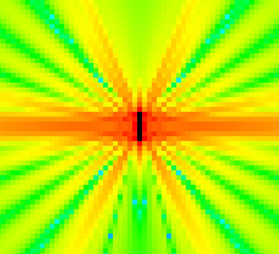
When that’s all done, we convert the final pressure to an SPL, which can be assigned a color.
When those colors are plotted, we have our acoustical calculation/ simulation to look at on the grid.