Tag Archives: Measurement

If You Can Hear It, You Can Measure It

Sound is a physical phenomenon, and is therefore quantifiable through measurement.

Please Remember:

The opinions expressed are mine only. These opinions do not necessarily reflect anybody else’s opinions. I do not own, operate, manage, or represent any band, venue, or company that I talk about, unless explicitly noted.

Want to use this image for something else? Great! Click it for the link to a high-res or resolution-independent version.

I’m going to start by saying this: Something being measurable does NOT require the exclusion of a sense of beauty, wonder, and awe about it. Measuring doesn’t destroy all that. It merely informs it.

The next thing I’m going to say is that it drives me CRAZY how, in an industry that is all physics all the time, we manage to convince ourselves that there are extra-logical explanations for “stuff sounding better.” Horsefeathers! If your ears detected a real difference – a difference not generated entirely by your mind – then that difference can be measured and quantified. Don’t get me wrong! It might be very hard to measure and quantify. Designing the experiment might very well be non-trivial. You might not know what you’re looking for. Your human hearing system might be able to deal with contaminants to the measurement that a single microphone might not handle well.

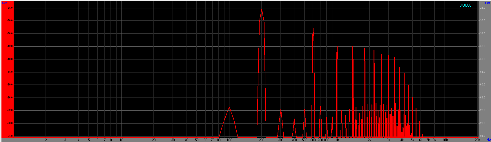
But whatever the difference is, if it’s real, it can definitely be described in terms of magnitude, frequency, and phase.

Take this statement: “We need to run the system through [x], because [person] ran their system through [x], and it all sounded a lot better.”

That’s fair to say. In this business, perception matters. But ask yourself, why did you like the system better when [x] was involved? There has to be a physical reason, assuming the system actually sounded different. If you deluded yourself into thinking there was a difference (because [x] is much more expensive than [y]), that’s a whole other discussion. Disregarding that possibility…

Did the system seem louder? As long as the overall SPL isn’t uncomfortable, and all other things are equal, audio humans tend to perceive a louder rig as being better. If something was actually louder, that can be measured. (Probably with tremendous ease and simplicity.)

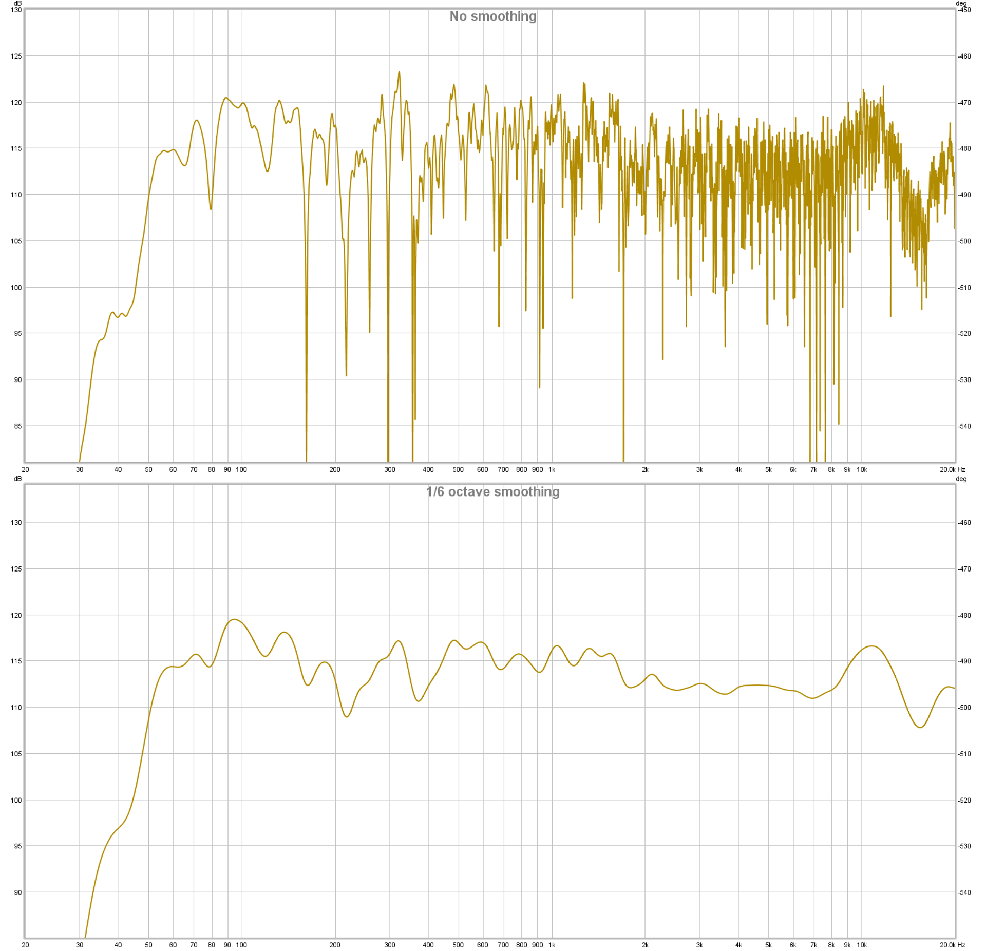
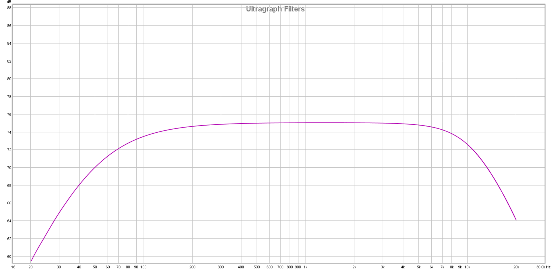
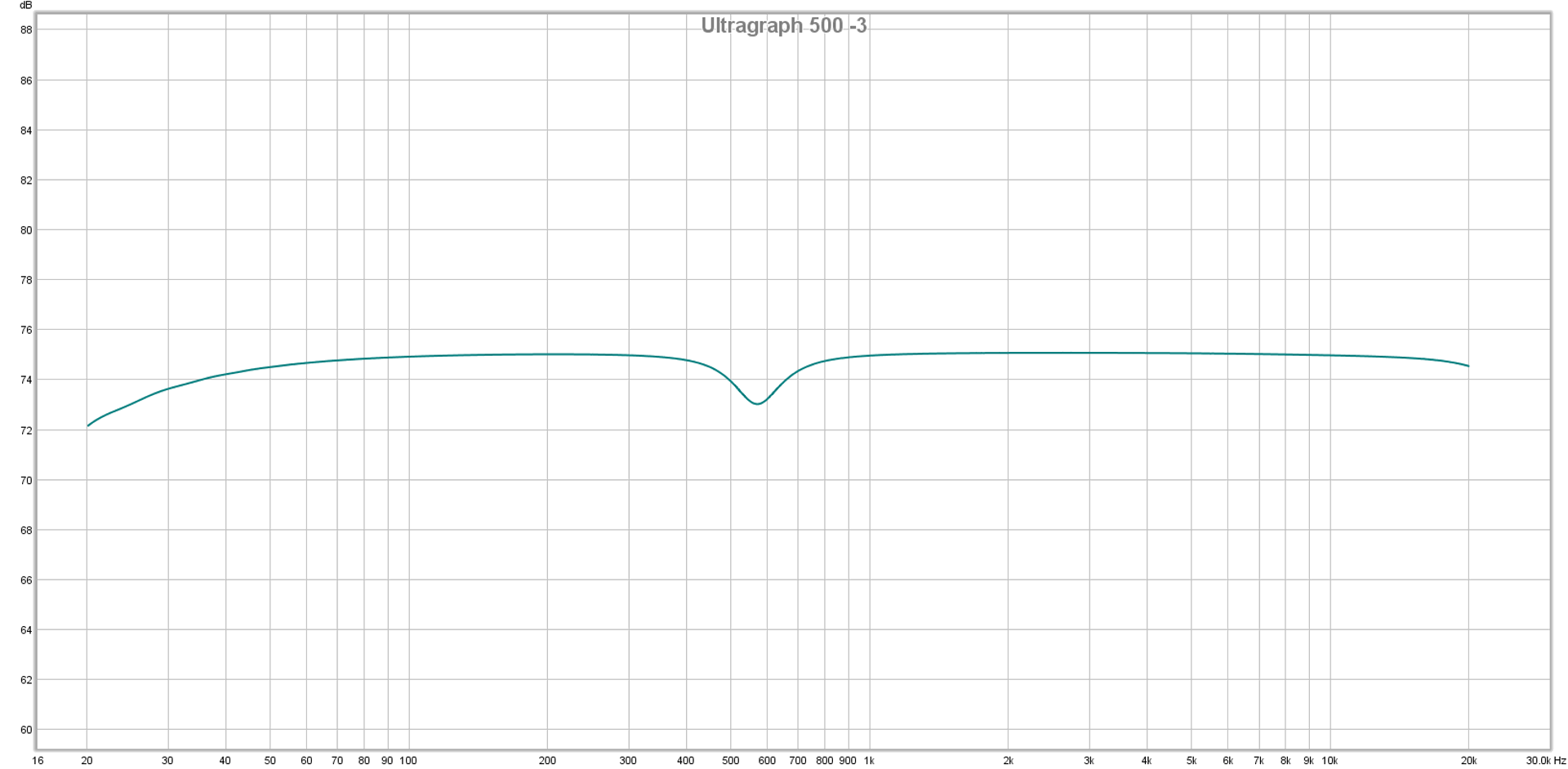
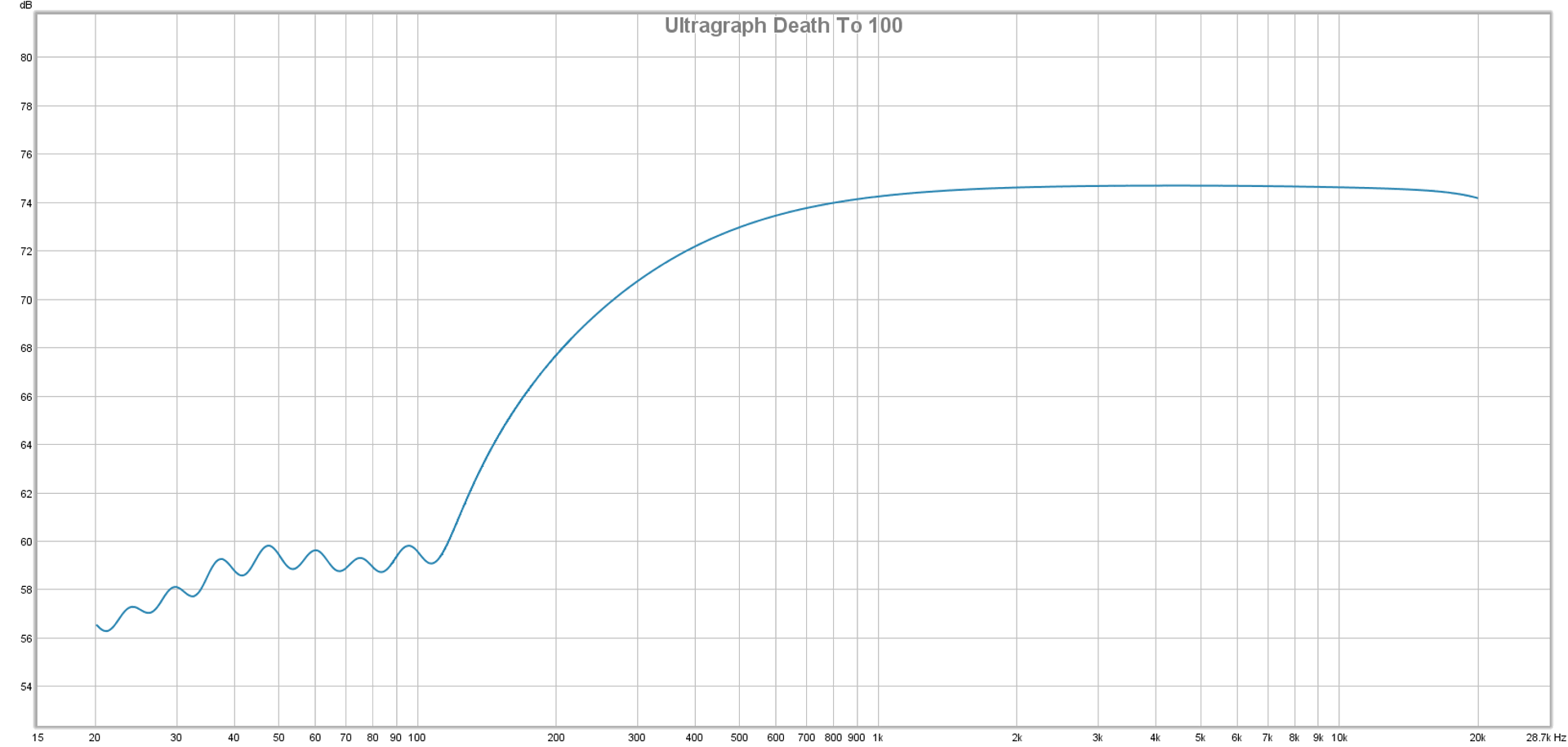
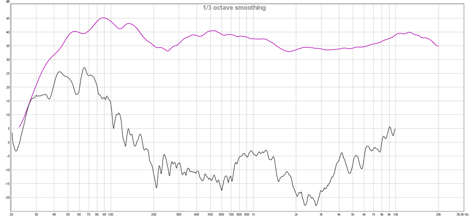
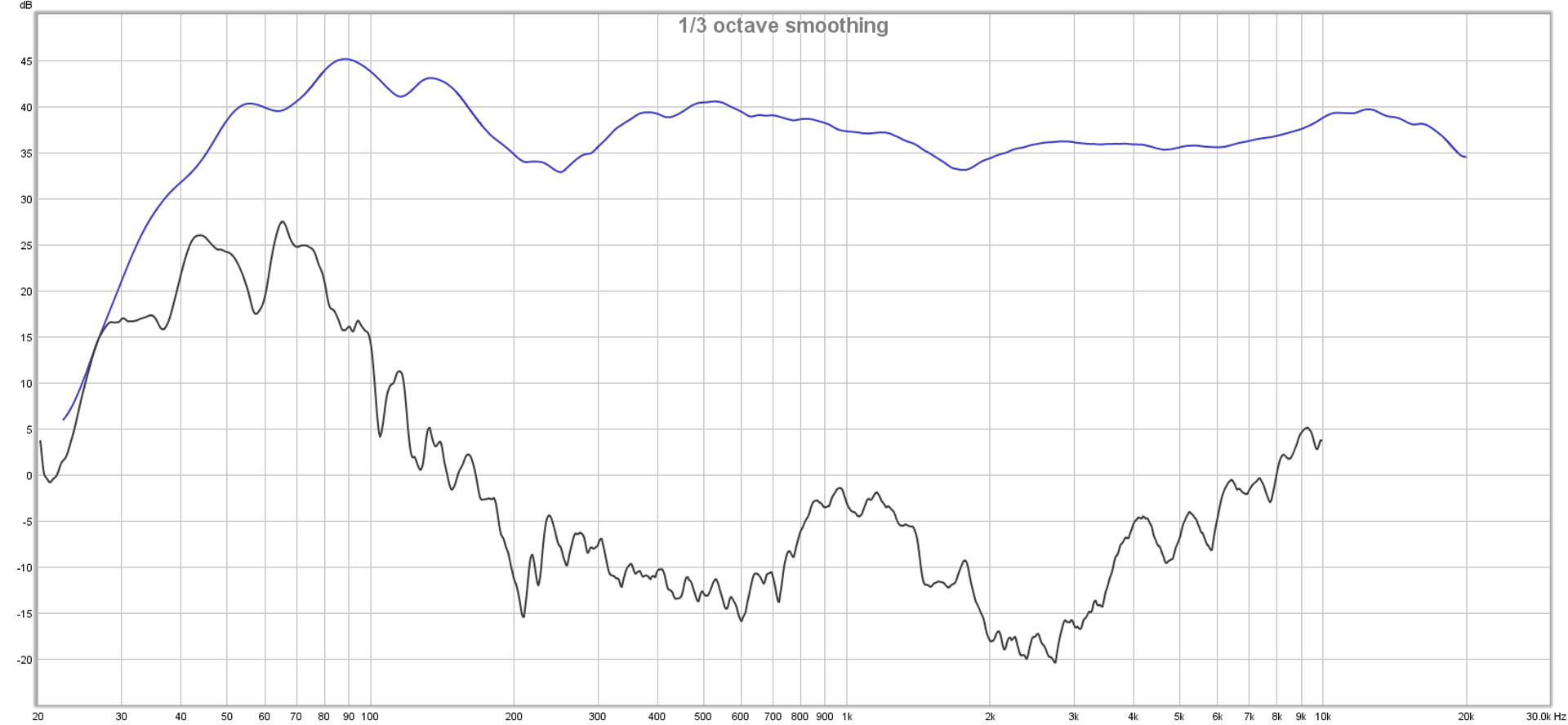
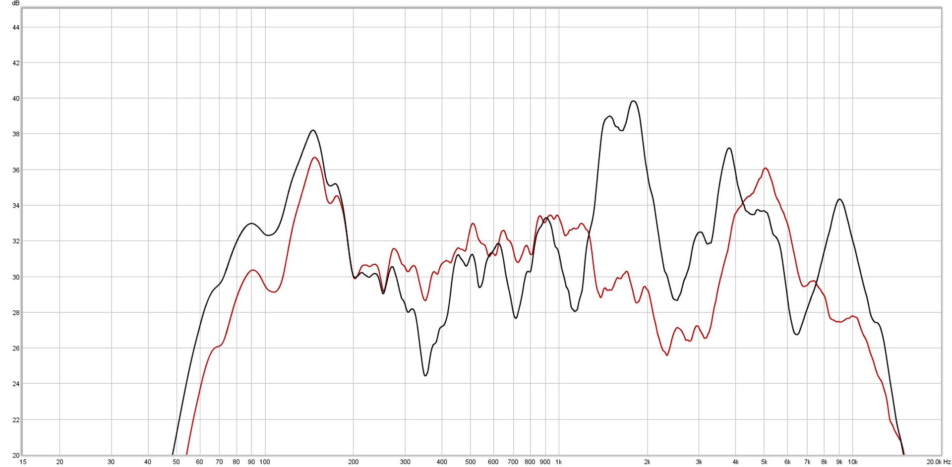
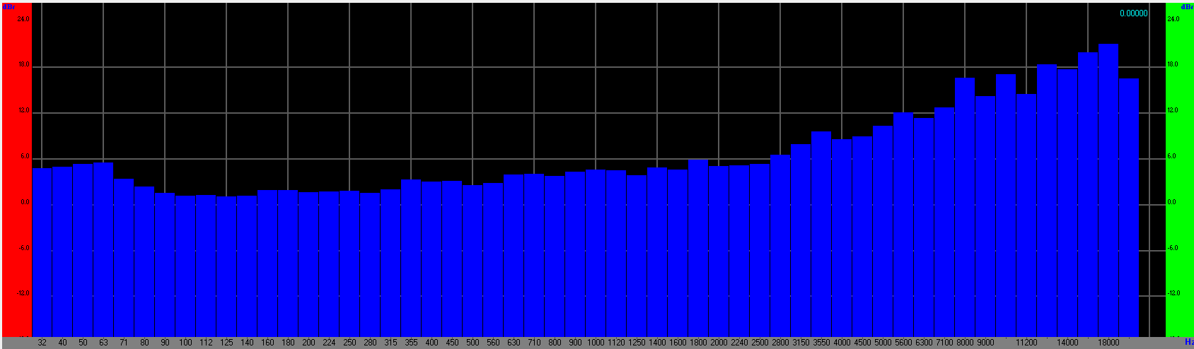
Maybe the basic system tuning solution created with [x] was just fundamentally better than what you’ve done with [y]. It’s entirely possible that you’ve gotten into a rut with the magnitude response that you tend to dial up with [y], and the other operator naturally arrives at something different. You like that something different. That something different is entirely measurable on a frequency response trace.

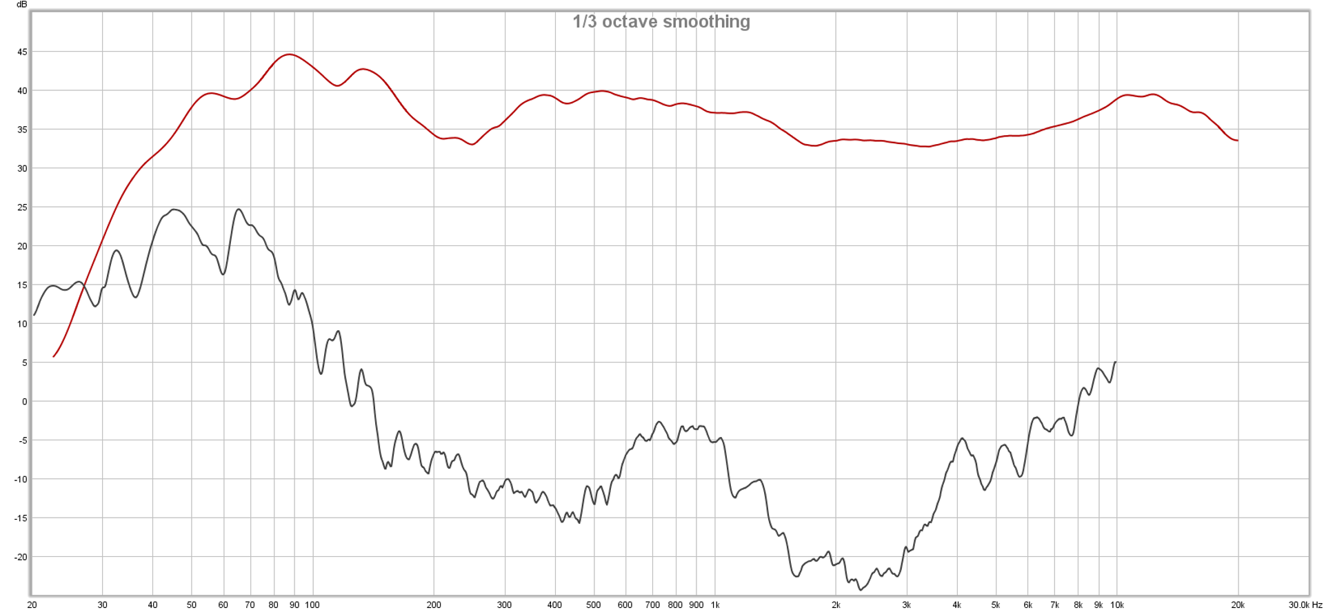
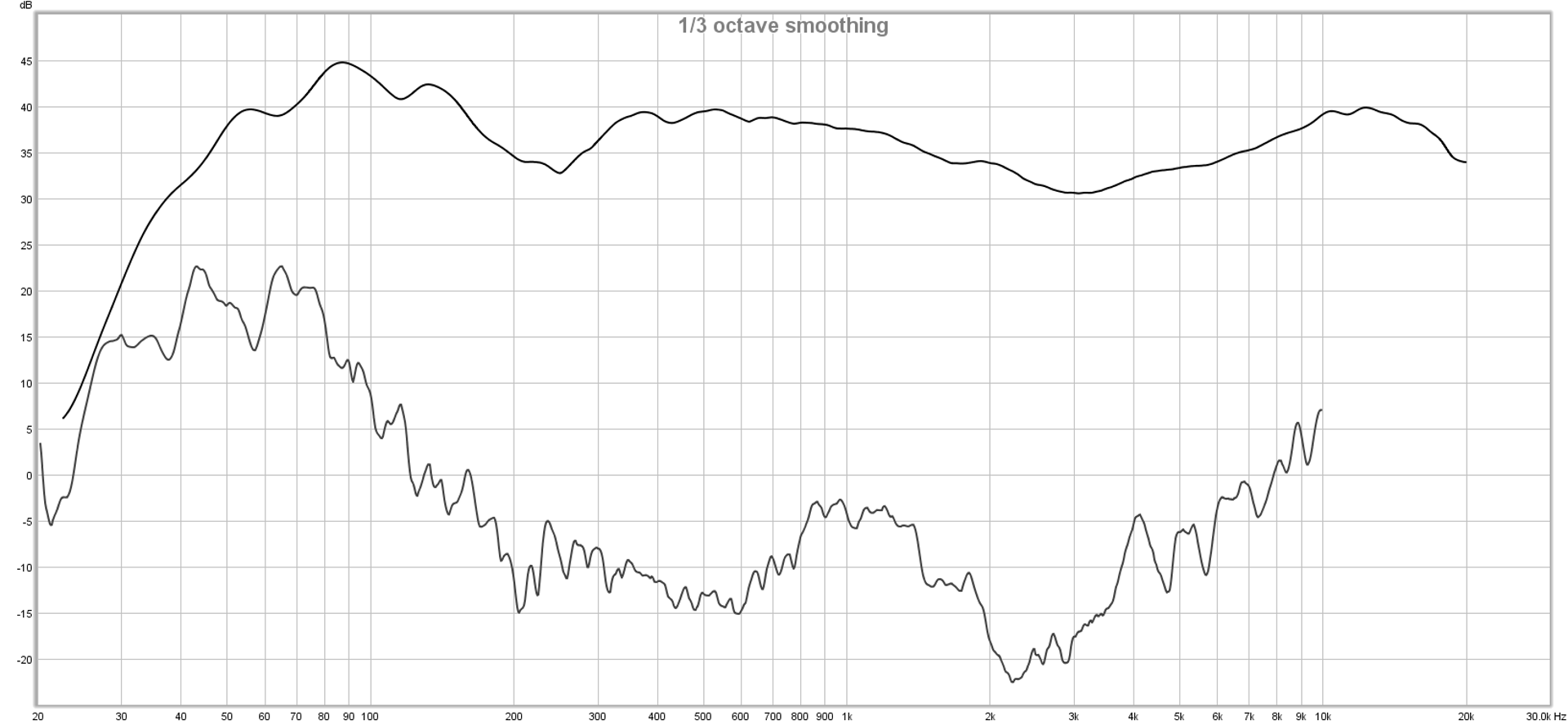
Maybe it wasn’t [x] at all. Maybe you were in a different room, and you liked the acoustics better. Maybe the different room has less “splatter,” or maybe it causes a low-frequency buildup that you enjoy. An RT60 measurement might reveal the difference, as might a waterfall plot, or maybe we’re right back to the basic magnitude vs. frequency trace again.

Maybe the deployment of the system was a little different, and a couple of boxes arrived and combined in a way you preferred. Maybe it’s time to look at your phase measurements…or frequency response, again, some more.

The basic human hearing input apparatus does not have capabilities which are difficult for modern technology to meet or exceed. If you’re reading this, you very probably can no longer hear the entire theoretical bandwidth that humans can handle. Measurement mics which can sense that entire bandwidth (and maybe more) can be had for less than $100 US. What can’t be easily replicated is the giant, pattern-synthesizing computer that we keep locked inside our skulls. That’s not really relevant, though, because imagination isn’t hearing. It’s imagination. Imagination can’t be measured, but real events in the world can be. What matters in audio, what we have a chance of controlling, are those real events.

Comparisons Of Some Powered Loudspeakers

Let’s measure some boxes!

Please Remember:

Want to use this image for something else? Great! Click it for the link to a high-res or resolution-independent version.

Over time, I’ve become more and more interested in how different products compare to each other in an objective sense. This is one reason why I put together the The Great, Quantitative, Live-Mic Shootout. What I’m especially intrigued about right now is loudspeakers – especially those that come packaged with their own internal amplification and DSP. Being able to quantify value for money in regards to these units seems like a nifty exercise, especially as there seems to be a significant amount of performance available at relatively low cost.

Over time, I’ve used a variety of powered loudspeakers in my work, and I have on hand a few different models. That’s why I tested what I tested – they were conveniently within reach!

Testing Notes

1) The measurement mic and loudspeaker under test were set up to mimic a situation where the listener was using the loudspeaker as a stage monitor.

2) A 1-second, looping, logarithmic sweep was used to determine the drive level where the loudspeaker’s electronics reached maximum output (meaning that a peak/ limit/ clip indicator clearly illuminated for roughly half a second).

3) Measurements underwent 1/6th octave smoothing for the sake of readability.

4) These comparisons are mostly concerned with a “music-critical band,” which I define as the range from 75 Hz to 10,000 Hz. This definition is based on the idea that the information required for both creating music live and enjoying reproduced sound is mostly contained within that passband.

5) “Volume” is the number of cubic inches contained within a rectangular prism just large enough to enclose the loudspeaker. (In other words, how big of a box just fits around the loudspeaker.)

6) “Flatness Deviation” is the difference in SPL between the lowest recorded level and highest recorded level in the music-critical band. A lower flatness deviation number indicates greater accuracy.

6) Similarly to #5, “Phase Flatness Deviation” is the difference between the highest phase and lowest phase degrees recorded in the music-critical band. (The phase trace is a generated, minimum-phase graph).

8) Distortion is the measured THD % at 1 kHz.

9) When available, in-box processing was set to be as minimal as possible (i.e., flat EQ).

Test Results And Comments (In Order Of Price)

Alto TS312

Acquisition Cost:	$299
Volume:	4565 in^3
Mass:	36 lbs
Magnitude And Phase:
Flatness Deviation:	12 dB
Phase Flatness Deviation:	166 degrees
Peak SPL:	119.6 dB
Distortion @ 1 kHz:	1.1%
Comments:	Good bang vs. buck ratio. Highly compact, competitive weight. Surprisingly decent performer, with respectable output and distortion characteristics. Lacks the “super-tuned” flatness of a Yamaha DBR, and not as clean as the JBL Eon. Simplified back panel lacks features, but also is hard to set incorrectly. Would have liked a “thru” option, but the push-button ability to lift signal ground is nice to have.

Peavey PVXP12

Acquisition Cost:	$399
Volume:	5917 in^3
Mass:	43 lbs
Magnitude And Phase:
Flatness Deviation:	14 dB
Phase Flatness Deviation:	230 degrees
Peak SPL:	123.8 dB
Distortion @ 1 kHz:	1.61%
Comments:	High output at limit, but the manufacturer allows for rather more distortion compared to other products. Not factory-tuned quite as flat as other boxes, with an output peak that reads well as a “single number” performance metric…but also sits in a frequency range that tends to be irritating at high volume and troublesome for feedback. The enclosure is hefty and bulky in comparison to similar offerings.

JBL Eon 612

Acquisition Cost:	$449
Volume:	4970 in^3
Mass:	33 lbs
Magnitude And Phase:
Flatness Deviation:	11 dB
Phase Flatness Deviation:	145 degrees
Peak SPL:	114.3 dB
Distortion @ 1 kHz:	0.596%
Comments:	Relatively low output, but also tuned to a more more flat solution than some (and with rather lower distortion). Has some compactness and weight advantages. Lots of digital bells and whistles, but the utility of the features varies widely across different user needs. (For instance, I would prefer trading more power and an even flatter tuning for the Bluetooth control connectivity.) Not particularly enamored of the “boot-up” time required for all the electronics to register as ready for operation.

Yamaha DBR 12

Acquisition Cost:	$499
Volume:	4805 in^3
Mass:	34.8 lbs
Magnitude And Phase:
Flatness Deviation:	10.6 dB
Phase Flatness Deviation:	180 degrees
Peak SPL:	119.5 dB
Distortion @ 1 kHz:	0.606%
Comments:	Good output at low distortion. Compact box in comparison to others. Competitive in terms of weight. Slightly more expensive than other offerings, commensurate with its improved performance. Measures very well in the “intelligibility zone” of its frequency response. Very pleased with the simple and robust selector switches for most operations.

In Defense Of Smoothing Your Traces

In the end, you have to be able to read a graph for the graph to be useful.

Please Remember:

Want to use this image for something else? Great! Click it for the link to a high-res or resolution-independent version.

There are people out there who insist that, when measuring an audio system, you should never smooth the trace. The argument is that you might miss some weird anomaly that gets filtered out by the averaging – and, in any case, the purpose of graphing a transfer function isn’t for the picture to look nice.

I think that’s an understandable sentiment, especially because it’s a thought uttered by people who I think are knowledgeable, respectable, and worth working alongside. At the same time, though, I can’t fully embrace their thinking. I very regularly apply 1/6th octave smoothing to measurements, and I do it for a very specific reason: I do indeed want to see the anomalies that matter, and I need to be able to clearly contextualize them.

The featured image on this article is an example of why I think the way I do. I’ve got a bit of a science-project going, and part of that project involved measuring a Yamaha DBR12. The traces you see in the picture are the same measurement, with the bottom one being smoothed. The unsmoothed trace is very hard to read for all the visual noise it presents, which makes it difficult to make any sort of decision about what corrections to make. the smoothed trace gives me a lot more to go on. I can see that 90 Hz – 150 Hz could come down a bit, with 2 kHz – 7.5 kHz maybe needing a bit of a bump to achieve maximum flatness.

So, I say, smooth those traces…but don’t oversmooth them! You want to suppress the information overload without losing the ability to find things that stand out. The 1/6th octave option seems to be the right compromise for me, with 1/12th still being more detail than is useful and 1/3rd getting into the area where too much gets lost.

And here’s another wrinkle: I support unsmoothed traces when you’re measuring devices that ignore acoustics, like the transfer function of a mixing console from input to output. In such a case, you should expect a very, very linear transfer function, and so the ability to spot tiny deviations is a must. The difficulty is when you’re in a situation where there a gazillion deviations, and they all appear significant. In such a case, which I’ve found to be the norm for measurements that involve acoustics, filtering to find what’s actually significant to the operation of an audio system is helpful.

Graphic Content

Transfer functions of various reasonable and unreasonable graphic EQ settings.

Please Remember:

Want to use this image for something else? Great! Click it for the link to a high-res or resolution-independent version.

An aphorism that I firmly believe goes like this: “If you can hear it, you can measure it.” Of course, there’s another twist to that – the one that reminds you that it’s possible to measure things you can’t hear.

The graphic equalizer, though still recognizable, is losing a bit of its commonality as an outboard device. With digital consoles invading en masse, making landings up and down the treasure-laden coasts of live audio, racks and racks of separate EQ devices are being virtualized inside computer-driven mix platforms. At the same time, hardware graphics are still a real thing that exists…and I would wager that most of us haven’t seen a transfer function of common uses (and abuses) of these units, which happen whether you’ve got a physical object or a digital representation of one.

So – let me dig up a spare Behringer Ultragraph Pro, and let’s graph a graphic. (An important note: Any measurement that you do is a measurement of EXACTLY that setup. Some parts of this exercise will be generally applicable, but please be aware that what we’re measuring is a specific Behringer EQ and not all graphic EQs in the world.)

The first thing to look at is the “flat” state. When you set the processing to “out,” is it really out?

In this case, very much so. The trace is laser flat, with +/- 0.2 dB of change across the entire audible spectrum. It’s indistinguishable from a “straight wire” measurement of my audio interface.

Now, we’ll allow audio to flow through the unit’s filtering, but with the high and low-pass filters swept to their maximums, and all the graph filters set to 0 dB.

The low and high-pass filters are still definitely having an effect in the audible range, though a minimal one. Half a decibel down at 45 Hz isn’t nothing, but it’s also pretty hard to hear.

What happens when the filters are swept to 75 Hz and 10 kHz?

The 3dB points are about where the labeling on the knobs tells you it should be (with a little bit of overshoot), and the filters roll off pretty gently (about 6 dB per octave).

Let’s sweep the filters out again, and make a small cut at 500 Hz.

Interestingly, the filter doesn’t seem to be located exactly where the faceplate says it should be – it’s about 40% of a third-octave space away from the indicated frequency center, if the trace is accurate in itself.

What if we drop the 500 Hz filter all the way down, and superimpose the new trace on the old one?

The filter might look a bit wider than what you expected, with easily measurable effects happening at a full octave below the selected frequency. Even so, that’s pretty selective compared to lots of wide-ranging, “ultra musical” EQ implementations you might run into.

What happens when we yank down two filters that are right next to each other?

There’s an interesting ripple between the cuts, amounting to a little bit less than 1 dB.

How about one of the classic graphic EQ abuses? Here’s a smiley-face curve:

Want to destroy all semblance of headroom in an audio system? It’s easy! Just kill the level of the frequency range that’s easiest to hear and most efficient to reproduce, then complain that the system has no power. No problem! :Rolls Eyes:

Here’s another EQ abuse, alternately called “Death To 100” or “I Was Too Cheap To Buy A Crossover:”

It could be worse, true, but…really? It’s not a true substitute for having the correct tool in the first place.

The Grand Experiment

A plan for an objective comparison of the SM58 to various other “live sound” microphones.

Please Remember:

Want to use this image for something else? Great! Click it for the link to a high-res or resolution-independent version.

Purpose And Explanation

Ever since The Small Venue Survivalist became a reality, I have wanted to do a big experiment. I’ve been itching to round up a bunch of microphones that can be purchased for either below, or slightly above the price point of the SM58, and then to objectively compare them to an SM58. (The Shure SM58 continues to be an industry standard microphone that is recognized and accepted everywhere as a sound-reinforcement tool.)

The key word above is “objectively.” Finding subjective microphone comparisons isn’t too hard. Sweetwater just put together (in 2017) a massive studio-mic shootout, and it was subjective. That is, the measurement data is audio files that you must listen to. This isn’t a bad thing, and it makes sense for studio mics – what matters most is how the mic sounds to you. Listening tests are everywhere, and they have their place.

In live audio, though, the mic’s sound is only one factor amongst many important variables. Further, these variables can be quantified. Resistance to mechanically-induced noise can be expressed as a decibel number. So can resistance to wind noise. So can feedback rejection. Knowing how different transducers stack up to one another is critical for making good purchasing decisions, and yet this kind of quantitative information just doesn’t seem to be available.

So, it seems that some attempt at compiling such measurements might be helpful.

Planned Experimental Procedure

Measure Proximity Effect

1) Generate a 100Hz tone through a loudspeaker at a repeatable SPL.

2) Place the microphone such that it is pointed directly at the center of the driver producing the tone. The front of the grill should be 6 inches from the loudspeaker baffle.

3) Establish an input level from the microphone, and note the value.

4) Without changing the orientation of the microphone relative to the driver, move the microphone to a point where the front of the grill is 1 inch from the loudspeaker baffle.

5) Note the difference in the input level, relative to the level obtained in step 3.

Assumptions: Microphones with greater resistance to proximity effect will exhibit a smaller level differential. Greater proximity effect resistance is considered desirable.

Establish “Equivalent Gain” For Further Testing

1) Place a monitor loudspeaker on the floor, and position the microphone on a tripod stand. The stand leg nearest the monitor should be at a repeatable distance, at least 1 foot from the monitor enclosure.

2) Set the height of the microphone stand to a repeatable position that would be appropriate for an average-height performer.

3) Changing the height of the microphone as little as possible, point the microphone directly at the center of the monitor.

4) Generate pink-noise through the monitor at a repeatable SPL.

5) Using a meter capable of RMS averaging, establish a -40 dBFS RMS input level.

Measure Mechanical Noise Susceptibility

1) Set the microphone such that it is parallel to the floor.

2) Directly above the point where the microphone grill meets the body, hold a solid, semi-rigid object (like an eraser, or small rubber ball) at a repeatable distance at least 1 inch over the mic.

3) Allow the object to fall and strike the microphone.

4) Note the peak input level created by the strike.

Assumptions: Microphones with greater resistance to mechanically induced noise will exhibit a lower input level. Greater resistance to mechanically induced noise is considered desirable.

Measure Wind Noise Susceptibility

1) Position the microphone on the stand such that it is parallel to the floor.

2) Place a small fan (or other source of airflow which has repeatable windspeed and air displacement volume) 6 inches from the mic’s grill.

3) Activate the fan for 10 seconds. Note the peak input level created.

Assumptions: Microphones with greater resistance to wind noise will exhibit a lower input level. Greater resistance to wind noise is considered desirable.

Measure Feedback Resistance

1) Set the microphone in a working position. For cardioid mics, the rear of the microphone should be pointed directly at the monitor. For supercardioid and hypercardioid mics, the the microphone should be parallel with the floor.

2a) SM58 ONLY: Set a send level to the monitor that is just below noticeable ringing/ feedback.

2b) Use the send level determined in 2a to create loop-gain for the microphone.

3) Set a delay of 1000ms to the monitor.

4) Begin a recording of the mic’s output.

5) Generate a 500ms burst of pink-noise through the monitor. Allow the delayed feedback loop to sound several times.

6) Stop the recording, and make note of the peak level of the first repeat of the loop.

Assumptions: Microphones with greater feedback resistance will exhibit a lower input level on the first repeat. Greater feedback resistance is considered desirable.

Measure Cupping Resistance

1) Mute the send from the microphone to the monitor.

2) Obtain a frequency magnitude measurement of the microphone in the working position, using the monitor as the test audio source.

3) Place a hand around as much of the mic’s windscreen as is possible.

4) Re-run the frequency magnitude measurement.

5) On the “cupped” measurement, note the difference between the highest response peak, and that frequency’s level on the normal measurement.

Assumptions: Microphones with greater cupping resistance will exhibit a smaller level differential between the highest peak of the cupped response and that frequency’s magnitude on the normal trace. Greater cupping resistance is considered desirable.

THD Troubleshooting

I might have discovered something, or I might not.

Please Remember:

Want to use this image for something else? Great! Click it for the link to a high-res or resolution-independent version.

Over the last little while, I’ve done some shows where I could swear that something strange was going on. Under certain conditions, like with a loud, rich vocal that had nothing else around it, I was sure that I could hear something in FOH distort.

So, I tried soloing up the vocal channel in my phones. Clean as a whistle.

I soloed up the the main mix. That seemed okay.

Well – crap. That meant that the problem was somewhere after the console. Maybe it was the stagebox output, but that seemed unlikely. No…the most likely problem was with a loudspeaker’s drive electronics or transducers. The boxes weren’t being driven into their limiters, though. Maybe a voice coil was just a tiny bit out of true, and rubbing?

Yeesh.

Of course, the very best testing is done “In Situ.” You get exactly the same signal to go through exactly the same gear in exactly the same place. If you’re going to reproduce a problem, that’s your top-shelf bet. Unfortunately, that’s hard to do right in the middle of a show. It’s also hard to do after a show, when Priority One is “get out in a hurry so they can lock the facility behind you.”

Failing that – or, perhaps, in parallel with it – I’m becoming a stronger and stronger believer in objective testing: Experiments where we use sensory equipment other than our ears and brains. Don’t get me wrong! I think ears and brains are powerful tools. They sometimes miss things, however, and don’t natively handle observations in an analytical way. Translating something you hear onto a graph is difficult. Translating a graph into an imagined sonic event tends to be easier. (Sometimes. Maybe. I think.)

This is why I do things like measure the off-axis response of a cupped microphone.

In this case, though, a simple magnitude measurement wasn’t going to do the job. What I really needed was distortion-per-frequency. Room EQ Wizard will do that, so I fired up my software, plugged in my Turbos (one at a time), and ran some trials. I did a set of measurements at a lower volume, which I discarded in favor of traces captured at a higher SPL. If something was going to go wrong, I wanted to give it a fighting chance of going wrong.

Here’s what I got out of the software, which plotted the magnitude curve and the THD curve for each loudspeaker unit:

I expected to see at least one box exhibit a bit of misbehavior which would dramatically affect the graph, but that’s not what I got. What I can say is that the first measurement’s overall distortion curve is different, lacking the THD “dip” at 200 Hz that the other boxes exhibit, significantly more distortion in the “ultra-deep” LF range, and with the “hump” shifted downwards. (The three more similar boxes center that bump in distortion at 1.2 kHz. The odd one out seems to put the center at about 800 Hz.)

So, maybe the box that’s a little different is my culprit. That’s my strong suspicion, anyway.

Or maybe it’s just fine.

Hmmmmm…

Measuring A Cupped Mic

What you might think would happen isn’t what happens.

Please Remember:

Want to use this image for something else? Great! Click it for the link to a high-res or resolution-independent version.

The most popular article on this site to date is the one where I talk about why cupping a vocal mic is generally a “bad things category” sort of experience. In that piece, I explain some general issues with wrapping one’s hand around a microphone grill, but there’s something I didn’t do:

I didn’t measure anything.

That reality finally dawned on me, so I decided to do a quck-n-dirty experiment on how a microphone’s transfer function changes when cupping comes into play. Different mics will do different things, so any measurement is only valid for one mic in one situation. However, even if the results can’t truly be generalized, they are illuminating.

In the following picture, the red trace is a mic pointing away from a speaker, as you would want to happen in monitor-world. The black trace is the mic in the same position, except with my hand covering a large portion of the windscreen mesh.

You would think that covering a large part of the mic’s business-end would kill off a lot of midrange and high-frequency information, but the measurement says otherwise. The high-mid and HF information is actually rather hotter, with large peaks at 1800 Hz, 3900 Hz, and 9000 Hz. The low frequency response below 200 Hz is also given a small kick in the pants. Overall, the microphone transfer function is “wild,” with more pronounced differences between peaks and dips.

The upshot? The transducer’s feedback characteristics get harder to manage, and the sonic characteristics of the unit begin to favor the most annoying parts of the audible spectrum.

Like I said, this experiment is only valid for one mic (a Sennheiser e822s that I had handy). At the same time, my experience is that other mics have “cupping behavior” which is not entirely dissimilar.

Single-Ended Measurement

I really prefer it over minutes on-end of loud pink-noise.

Please Remember:

Want to use this image for something else? Great! Click it for the link to a high-res or resolution-independent version.

Today, I helped teach a live-sound class at Broadview Entertainment Arts University. We put a stage together, ran power, and set both Front Of House (FOH) and monitor-world loudspeakers. To cap-off the day, I decided to show the students a bit about measuring and tuning the boxes that we had just finished squaring away.

The software we used was Room EQ Wizard.

The more I use “REW,” the more I like the way it works. Its particular mode of operation isn’t exactly industry-standard, but I do have a tendency to ignore the trends when they aren’t really helpful or interesting to me. Rather than continually blasting pink-noise (statistically uncorrelated audio signals with equal energy per octave from 20 Hz to 20 kHz) into a room for several minutes while you tweak your EQ, Room EQ Wizard plays a predetermined sine-sweep. It then shows you a graph, you make your tweaks based on the graph, you re-measure, and iterate as many times as needed.

I prefer this workflow for more than one reason.

Single Ended Measurements Are Harder To Screw Up

The industry-standard method for measuring and tuning loudspeakers is that of the dual-FFT. If you’ve used or heard of SysTune or SMAART, among others, those are dual-FFT systems. You run an essentially arbitrary signal through your rig, with that signal not necessarily being “known” ahead of time. That signal has to be captured at two points:

1) Before it enters the signal chain you actually want to test.

2) After it exits the signal chain in question.

And, of course, you have to compensate for any propagation delay between those two points. Otherwise, your measurement will get contaminated with statistical “noise,” and become harder to read in a useful way – especially if phase matters to you. Averaging does help with this, to be fair, and I do average my “REW” curves to make them easier to parse. Anybody who has taken and examined a measurement trace in a real room knows that unsmoothed results look pretty terrifying.

In any event, dual-FFT measurements tend to be more difficult to set up and run effectively. On top of how easy it is to screw up ANY measurement, whether by measuring the wrong thing, forgetting an upstream EQ, or putting the mic in a terrible spot, you have the added hassles of getting your two measurement points routed and delay-compensated.

Over the years, dual-FFT packages have gotten much better at guiding users through the process, internally looping back the reference signal, and automatically picking compensation delay times. Even so, automating a complicated process doesn’t make the process less complicated. It just shields you from the complexity for as long as the automation can help you. (I’m not bagging on SMAART and SysTune here. They’re good bits of software that plenty of folks use successfully. I’m just pointing some things out.)

Single Ended, “Sweep” Measurements Can Be Quieter (And Less Annoying)

Another issue with measurements involving broadband signals is that they have greater susceptibility to in-room noise. As a whole, the noise may be quite loud. However, any given frequency can’t be running very “hot,” as the entire signal has to make it cleanly through the signal path. As such, noise in the room easily contaminates the test at the frequencies contained within that noise, unless you run the test signal loudly enough. With a single-ended, sine-sweep measurement, the instant that the measurement tone is at a certain frequency, the entire system output is dedicated to that frequency alone. As such, if you have in-room noise of 50 dB SPL at 1 kHz, running your measurement signal at 70 dB SPL should completely blow past the noise – while remaining comfortable to hear. With broadband noise, the measurement signal in the same situation might have to be 90 dB SPL.

Please note that single-ended measurements of broadband signals DO exist, and they have similar problems with noise as compared to broadband-noise, dual-FFT solutions.

The other nice thing about “sweep” measurements is that everybody gets a break from the noise. For 10 seconds or so, a rising tone sounds through the system, and then it stops. This is a stark contrast to minutes of “KSSSSSHHHHHH” that otherwise have to be endured.

Quality, Single Ended Measurement Software Can Be Cheaper

A person could conceivably design and build single-ended measurement software, and then sell it for a large amount of money. A person could also create dual-FFT software and give it away for free (Visual Analyzer is a good example).

However, on average, it seems that when it comes time to bring “easy to use” and “affordable” together, single-ended is where you’ll have to look. I really like Visual Analyzer, but you really, really have to know what you’re doing to use it effectively. SMAART and SysTune are user-friendly while also being incredibly powerful, but cost $700 – $1000 to acquire.

Room EQ Wizard is friendly (at least to me), and free. It’s hard to beat free when it’s also good.

I want to be careful to say (again) that I’m not trying to get people away from the highly-developed and widely accepted toolsets available in dual-FFT measurement packages. What I’m trying to say is that “dual-FFT with broadband noise in pseudo-realtime” isn’t the only way to measure and tune a sound system. There are other options that are easier to get into, and you can always step up later.

How Much Light For Your Dollar?

Measurements and observations regarding a handful of relatively inexpensive LED PARs.

Please Remember:

Want to use this image for something else? Great! Click it for the link to a high-res or resolution-independent version.

I’m in the process of getting ready for a pretty special show. The album “Clarity” by Sons Of Nothing is turning 10, and a number of us are trying to put together one smasher of a party.

Of course, that means video.

And our master of all things videographic is concerned about having enough light. We can’t have anybody in the band who’s permanently stuck in “shadow.” You only get one chance to shoot a 10th anniversary concert, and we want to get it right.

As such, I’m looking at how to beef up my available lighting instruments. It’s been a long while since I’ve truly gone shopping for that old mainstay of small-venue lighting, the LED wash PAR, but I do take a look around every so often. There’s a lot to see, and most of it isn’t very well documented. Lighting manufacturers love to tell you how many diodes are in a luminaire, and they also like to tell you how much power the thing consumes, but there appears to be something of an allergy to coughing up output numbers.

Lux, that is. Lumens per square meter. The actual effectiveness of a light at…you know…LIGHTING things.

So, I thought to myself, “Self, wouldn’t it be interesting to buy some inexpensive lights and make an attempt at some objective measurement?”

I agreed with myself. I especially agreed because Android 4.4 devices can run a cool little Google App called “Science Journal.” The software translates the output from a phone’s ambient light sensor into units of lux. For free (plus the cost of the phone, of course). Neat!

I got onto Amazon, found myself a lighting brand (GBGS) that had numerous fixtures available for fulfillment by Amazon, and spent a few dollars. The reason for choosing fulfillment from Amazon basically comes down to this: I wanted to avoid dealing with an unknown in terms of shipping time. Small vendors can sometimes take a while to pack and ship an order. Amazon, on the other hand, is fast.

The Experiment

Step 1: Find a hallway that can be made as dark as possible – ideally, dark enough that a light meter registers 0 lux.

Step 2: At one end, put the light meter on a stand. (A mic stand with a friction clip is actually pretty good at holding a smartphone, by the way.)

Step 3: At the other end, situate a lighting stand with the “fixture under test” clamped firmly to that stand.

Step 4: Measure the distance from the lighting stand to the light meter position. (In my case, the distance was 19 feet.)

Step 5: Darken the hallway.

Step 6: Set the fixture under test to maximum output using a DMX controller.

Step 7: Allow the fixture to operate at full power for roughly 10 minutes, in case light output is reduced as the fixture’s heat increases.

Step 8: Ensure the fixture under test is aimed directly at the light meter.

Step 9: Note the value indicated by the meter.

Important Notes

A relatively long distance between the light and the meter is recommended. This is so that any positioning variance introduced by placing and replacing either the lights or the meter has a reduced effect. At close range, a small variance in distance can skew a measurement noticeably. At longer distances, that same variance value has almost no effect. A four-inch length difference at 19 feet is about a 2% error, whereas that same length differential at 3 feet is an 11% error.

It’s important to note that the hallway used for the measurement had white walls. This may have pushed the readings higher, as – similarly to audio – energy that would otherwise be lost to absorption is re-emitted and potentially measurable.

It was somewhat difficult to get a “steady” measurement using the phone as a meter. As such, I have estimated lux readings that are slightly lower than the peak numbers I observed.

These fixtures may or may not be suitable for your application. These tests cannot meaningfully speak to durability, reliability, acceptability in a given setting, and so on.

The calculation for 1 meter lux was as follows:

19′ = 5.7912 m

5.7912 = 2^2.53 (2.53 doublings of distance from 1m)

Assumed inverse square law for intensity; For each doubling of distance, intensity quadruples.

Multiply 19′ lux by 4^2.53 (33.53)

Calculated 1 meter lux values are just that – calculated. LED PAR lights are not a point-source of light, and so do not behave like one. It requires a certain distance from the fixture for all the emitters to combine and appear as though they are a single source of light.

The Data

The data display requires Javascript to work. I’m sorry about that – I personally dislike it when sites can’t display content without Javascript. However, for the moment I’m backed into a corner by the way that WordPress works with PHP, so Javascript it is.

Ascending sort by:

Why Chaining Distortion Doesn’t Sound So Great

More dirt is not necessarily cool dirt.

Please Remember:

Want to use this image for something else? Great! Click it for the link to a high-res or resolution-independent version.

One day, just before Fats closed, I was talking with Christian from Blue Zen. We were discussing the pursuit of tone, and a discovery that Christian had made (with the help of Gary at Guitar Czar). Christian had been trying to get more drive from his amp, which already had a fair bit of crunch happening. So, he had put a distortion pedal between the guitar and the amplifier input.

He hadn’t liked the results. He found the sound to be too scratchy and thin.

Upon consultation with Gary, the distortion pedal had been removed, and a much cleaner boost substituted. Christian was definitely happier.

But why hadn’t the original solution worked?

The Frequency Domain

Distortion can be something of a complex creature, but it does have a “simple” form. The simple form is harmonic distortion. Harmonic distortion occurs when the transfer function of an audio chain becomes nonlinear, and a tone is passed with additional products that follow a mathematical pattern: For a given frequency in a signal, the generated products are integer multiples of that frequency.

Integers are “whole” numbers, so, for a 200 Hz tone undergoing harmonic distortion, additional tones are generated at 200 Hz X 2, 3, 4, 5, 6, etc. Different circuits generate the additional tones at different intensities, and which pattern you prefer is a matter of taste.

For example, here’s an RTA trace of a 200 Hz tone being run through a saturation plugin.

(The odd-numbered harmonics are definitely favored by this particular saturation processor’s virtual circuit.)

The thing is that harmonics are always higher in frequency than the fundamental. The “hotter” the harmonic content, the more the signal’s overall frequency response “tilts” toward the high end. As distortion piles up, the overall timbre of a signal can start to overwhelm the lower-frequency information, resulting in a sound that is no longer “warm,” “thick,” “fat,” “chunky,” “creamy,” or whatever adjective you like to use.

Take a look at this transfer function trace comparing a signal run through one distortion stage and two distortion stages. The top end is very pronounced, with plenty of energy that’s not much more than “fizz” or “hiss”:

If you chain distortion into distortion, you’re quite likely to just pile up more and more harmonic content, thus emphasizing the high end more than you’d prefer. There’s more to it than that, though. Look at this RTA trace of a tone being run through chained saturation plugins:

To make things easier to see, you can also take a look at this overlay of the two traces:

There’s noticeably more energy in the high-end, and the distortion products are also present at many more frequencies. The original harmonic distortion tones are being distorted themselves, and there may also be some intermodulation distortion occurring. Intermodulation distortion is also a nonlinearity in a system’s transfer function, but the additional tones aren’t multiples of the original tones. Rather, they are sums and differences.

IM distortion is generally thought to sound pretty ugly when compared to harmonic distortion.

So, yes, chaining distortion does give you more drive, but it can also give you way more “dirt” than you actually want. If you like the sound of your amp’s crunch, and want more of it, you’re better off finding a way to run your clean signal at a higher (but still clean) level. As the amp saturates, the distortion products will go up – but at least it will be only one set of distortion products.

Dynamic Range

The other problem with heaping distortion on top of distortion is that of emphasizing all kinds of noises that you’d prefer not to. Distortion is, for all intents and purposes, a “dirty” limiter. Limiting, being an extreme form of compression, reduces dynamic range (the difference between high and low amplitude signals). This can be very handy up to a point. Being able to crank up quieter sounds means that tricks like high-speed runs and pinch-harmonics are easier to pull off effectively.

There’s a point, though, where sounds that you’d prefer to de-emphasize are smashed right up into the things you do want to hear. To use a metaphor, the problem with holding the ceiling steady and raising the floor is that you eventually get that nasty old carpet in your face. The noise of your pickups and instrument processors? Loud. Your picking? Loud. Your finger movement on the strings? Loud. Any other sloppiness? Loud.

Running distortion into distortion is a very effective way to make what you’d prefer to be quiet into a screaming vortex of noise.

Is Chaining Distortion Wrong?

I want to close with this point.

Chaining distortion is not “wrong.” You shouldn’t be scared to try it as a science experiment, or to get a wild effect.

The point of all this is merely to say that serial distortion is not the best practice for a certain, common application – the application of merely running a given circuit at a higher level. For that particular result, which is quite commonly desired, you will be far better served by feeding the circuit with more “clean” gain. In all likelihood, your control over your sound will be more fine-grained, and also more predictable overall.